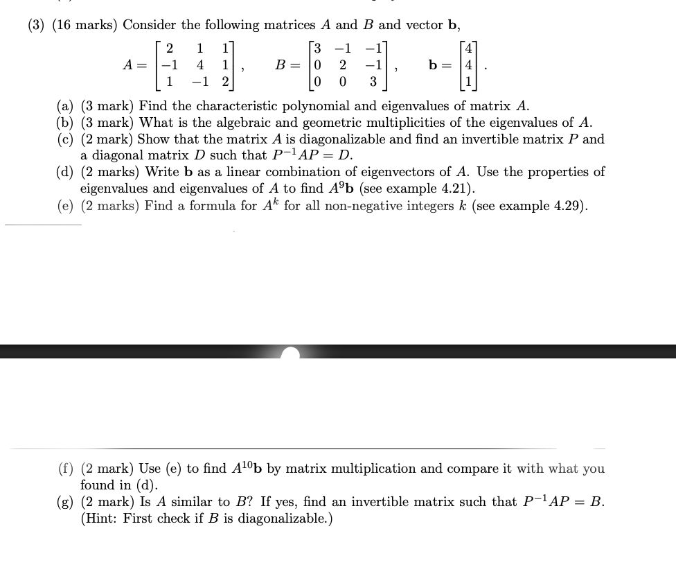
give answer in 2 step with explanation at the end of each step and final answer at the end:(3) (16 marks) Consider the following matrices A and B and vector b,
2 1 1 3 —1 —1 4
A=|-1 4 1|, B=|0o 2 -1|, b=|4].
1-12 00 3 1
(a) (3 mark) Find the characteristic polynomial and eigenvalues of matrix A.
(b) (3 mark) What is the algebraic and geometric multiplicities of the eigenvalues of A.
(¢) (2 mark) Show that the matrix A is diagonalizable and find an invertible matrix P and
a diagonal matrix D such that P~1AP = D.
(d) (2 marks) Write b as a linear combination of eigenvectors of A. Use the properties of
eigenvalues and eigenvalues of A to find A%b (see example 4.21).
(¢) (2 marks) Find a formula for A* for all non-negative integers k (sec example 4.29).
_________________a
(£) (2 mark) Use (¢) to find A'%b by matrix multiplication and compare it with what you
found in (d).
(g) (2 mark) Is A similar to B? If yes, find an invertible matrix such that P~AP = B.
(Hint: First check if B is diagonalizable.)
Question:
give answer in 2 step with explanation at the end of each step and final answer at the end:(3) (16 marks) Consider the following matrices A and B and vector b,
2 1 1 3 —1 —1 4
A=|-1 4 1|, B=|0o 2 -1|, b=|4].
1-12 00 3 1
(a) (3 mark) Find the characteristic polynomial and eigenvalues of matrix A.
(b) (3 mark) What is the algebraic and geometric multiplicities of the eigenvalues of A.
(¢) (2 mark) Show that the matrix A is diagonalizable and find an invertible matrix P and
a diagonal matrix D such that P~1AP = D.
(d) (2 marks) Write b as a linear combination of eigenvectors of A. Use the properties of
eigenvalues and eigenvalues of A to find A%b (see example 4.21).
(¢) (2 marks) Find a formula for A* for all non-negative integers k (sec example 4.29).
_________________a
(£) (2 mark) Use (¢) to find A'%b by matrix multiplication and compare it with what you
found in (d).
(g) (2 mark) Is A similar to B? If yes, find an invertible matrix such that P~AP = B.
(Hint: First check if B is diagonalizable.)
This is AI generated Response.
Asked by: Pagal
Created at: 2025-07-28 09:30:50
Final Answer:
RenderedRaw Text
Did you like this answer?
Sure! Let's tackle part (a) in two steps, as you requested.
---
## (a) Find the characteristic polynomial and eigenvalues of matrix \( A \).
### **Step 1: Find the characteristic polynomial of \( A \).**
The characteristic polynomial of a matrix \( A \) is defined as \( \det(A - \lambda I) \).
Given:
\[
A = \begin{bmatrix}
2 & 1 & 1 \\
-1 & 4 & 1 \\
1 & -1 & 2
\end{bmatrix}
\]
Subtract \( \lambda \) from the diagonal entries:
\[
A - \lambda I = \begin{bmatrix}
2-\lambda & 1 & 1 \\
-1 & 4-\lambda & 1 \\
1 & -1 & 2-\lambda
\end{bmatrix}
\]
Now, compute the determinant:
\[
\begin{align*}
\det(A - \lambda I) &=
\begin{vmatrix}
2-\lambda & 1 & 1 \\
-1 & 4-\lambda & 1 \\
1 & -1 & 2-\lambda
\end{vmatrix} \\
&= (2-\lambda)\begin{vmatrix}4-\lambda & 1 \\ -1 & 2-\lambda \end{vmatrix}
- 1\begin{vmatrix}-1 & 1 \\ 1 & 2-\lambda\end{vmatrix}
+ 1\begin{vmatrix}-1 & 4-\lambda \\ 1 & -1\end{vmatrix}
\end{align*}
\]
Calculate each minor:
- \( (4-\lambda)(2-\lambda) - (1)(-1) = (4-\lambda)(2-\lambda) + 1 \)
- \( (-1)(2-\lambda) - (1)(1) = -(2-\lambda) - 1 = -2 + \lambda - 1 = \lambda - 3 \)
- \( (-1)(-1) - (4-\lambda)(1) = 1 - (4-\lambda) = \lambda - 3 \)
Plug in the values:
\[
\begin{align*}
\det(A - \lambda I) &= (2-\lambda)[(4-\lambda)(2-\lambda) + 1] - 1[\lambda-3] + 1[\lambda-3] \\
&= (2-\lambda)[(4-\lambda)(2-\lambda) + 1] \\
\end{align*}
\]
Now, expand \( (4-\lambda)(2-\lambda) = 8 - 4\lambda - 2\lambda + \lambda^2 = 8 - 6\lambda + \lambda^2 \)
So,
\[
(4-\lambda)(2-\lambda) + 1 = (8 - 6\lambda + \lambda^2) + 1 = 9 - 6\lambda + \lambda^2
\]
Now, multiply:
\[
\det(A - \lambda I) = (2-\lambda)(9 - 6\lambda + \lambda^2)
\]
Expand:
\[
(2-\lambda)(\lambda^2 - 6\lambda + 9) = 2(\lambda^2 - 6\lambda + 9) - \lambda(\lambda^2 - 6\lambda + 9)
\]
\[
= 2\lambda^2 - 12\lambda + 18 - (\lambda^3 - 6\lambda^2 + 9\lambda)
\]
\[
= 2\lambda^2 - 12\lambda + 18 - \lambda^3 + 6\lambda^2 - 9\lambda
\]
\[
= -\lambda^3 + 8\lambda^2 - 21\lambda + 18
\]
**Explanation:**
We subtracted \(\lambda\) from the diagonal entries of \(A\), calculated the determinant, and expanded to obtain the characteristic polynomial.
**Characteristic Polynomial:**
\[
\boxed{-\lambda^3 + 8\lambda^2 - 21\lambda + 18}
\]
---
### **Step 2: Find the eigenvalues of \( A \).**
The eigenvalues are the roots of the characteristic polynomial:
\[
-\lambda^3 + 8\lambda^2 - 21\lambda + 18 = 0
\]
Or,
\[
\lambda^3 - 8\lambda^2 + 21\lambda - 18 = 0
\]
Let’s try rational roots (factors of 18): \( \pm1, \pm2, \pm3, \pm6, \pm9, \pm18 \).
Try \(\lambda = 1\):
\( 1 - 8 + 21 - 18 = -4 \) (not zero)
Try \(\lambda = 2\):
\( 8 - 32 + 42 - 18 = (8 - 32) + (42 - 18) = -24 + 24 = 0 \)
So, \(\lambda = 2\) is a root.
Now, perform synthetic or polynomial division to factor out \((\lambda - 2)\):
Divide \( \lambda^3 - 8\lambda^2 + 21\lambda - 18 \) by \( (\lambda - 2) \):
\[
\lambda^3 - 8\lambda^2 + 21\lambda - 18 = (\lambda - 2)(\lambda^2 - 6\lambda + 9)
\]
Factor \( \lambda^2 - 6\lambda + 9 = (\lambda - 3)^2 \)
So, characteristic equation factors as:
\[
(\lambda - 2)(\lambda - 3)^2 = 0
\]
So, eigenvalues are:
\[
\boxed{2, 3, 3}
\]
**Explanation:**
We solved the cubic polynomial and factored it to find the eigenvalues.
---
## **Final Answers for (a):**
- **Characteristic polynomial:** \( \boxed{-\lambda^3 + 8\lambda^2 - 21\lambda + 18} \)
- **Eigenvalues:** \( \boxed{2, 3, 3} \)
---
Would you like to proceed to (b)?
Question:
B
This is AI generated Response.
Asked by: Pagal
Created at: 2025-07-28 09:31:24
Final Answer:
RenderedRaw Text
Did you like this answer?
Certainly! Let's proceed to part (b) with two detailed steps, including explanations.
---
## (b) What are the algebraic and geometric multiplicities of the eigenvalues of \(A\)?
### **Step 1: Determine the algebraic multiplicities of each eigenvalue.**
From part (a), the eigenvalues are:
- \(\lambda = 2\)
- \(\lambda = 3\) (with multiplicity 2)
**Algebraic multiplicity** is the multiplicity of each eigenvalue as a root of the characteristic polynomial.
- \(\lambda = 2\) appears once, so **algebraic multiplicity** of 2 is **1**.
- \(\lambda = 3\) appears twice, so **algebraic multiplicity** of 3 is **2**.
**Explanation:**
Eigenvalues' algebraic multiplicities are obtained directly from the roots of the characteristic polynomial.
---
### **Step 2: Find the geometric multiplicities by computing the dimension of the eigenspaces.**
The **geometric multiplicity** of an eigenvalue is the dimension of the null space (kernel) of \(A - \lambda I\).
---
**For \(\lambda = 2\):**
Calculate \(A - 2I\):
\[
A - 2I = \begin{bmatrix}
2-2 & 1 & 1 \\
-1 & 4-2 & 1 \\
1 & -1 & 2-2
\end{bmatrix} = \begin{bmatrix}
0 & 1 & 1 \\
-1 & 2 & 1 \\
1 & -1 & 0
\end{bmatrix}
\]
Solve \((A - 2I)\mathbf{x} = 0\):
Row reduce:
\[
\begin{bmatrix}
0 & 1 & 1 \\
-1 & 2 & 1 \\
1 & -1 & 0
\end{bmatrix}
\]
Swap row 1 with row 3 to get a leading 1:
\[
\begin{bmatrix}
1 & -1 & 0 \\
-1 & 2 & 1 \\
0 & 1 & 1
\end{bmatrix}
\]
Add row 1 to row 2:
\[
\text{Row 2} = \text{Row 2} + \text{Row 1} \Rightarrow
[-1+1, 2+(-1), 1+0] = [0, 1, 1]
\]
Now the matrix:
\[
\begin{bmatrix}
1 & -1 & 0 \\
0 & 1 & 1 \\
0 & 1 & 1
\end{bmatrix}
\]
Subtract row 2 from row 3:
\[
\text{Row 3} - \text{Row 2} = [0, 1-1, 1-1] = [0, 0, 0]
\]
The augmented matrix indicates:
- \(x_1 - x_2 = 0 \Rightarrow x_1 = x_2\)
- \(x_2 + x_3 = 0 \Rightarrow x_3 = -x_2\)
Let \(x_2 = t\), then:
\[
x_1 = t,\quad x_3 = -t
\]
Eigenvector corresponding to \(\lambda=2\):
\[
\mathbf{x} = t \begin{bmatrix} 1 \\ 1 \\ -1 \end{bmatrix}
\]
**Dimension of eigenspace:** 1 (since only one free parameter)
**Therefore,** the **geometric multiplicity** of \(\lambda=2\) is **1**.
---
**For \(\lambda = 3\):**
Calculate \(A - 3I\):
\[
A - 3I = \begin{bmatrix}
-1 & 1 & 1 \\
-1 & 1 & 1 \\
1 & -1 & -1
\end{bmatrix}
\]
Solve \((A - 3I)\mathbf{x} = 0\):
Observe rows:
- Rows 1 and 2 are identical.
- Row 3 is \(-\) row 1.
Reduce:
\[
\begin{bmatrix}
-1 & 1 & 1 \\
-1 & 1 & 1 \\
1 & -1 & -1
\end{bmatrix}
\]
Replace row 3 with row 3 + row 1:
\[
[1 + (-1), -1 + 1, -1 + 1] = [0, 0, 0]
\]
So, the system reduces to two equations:
\[
-1 x_1 + 1 x_2 + 1 x_3 = 0
\]
and the second identical.
Express \(x_1\):
\[
x_1 = x_2 + x_3
\]
Choose free parameters \(x_2 = s\), \(x_3 = t\), then:
\[
x_1 = s + t
\]
Eigenvectors:
\[
\mathbf{x} = s \begin{bmatrix} 1 \\ 1 \\ 0 \end{bmatrix} + t \begin{bmatrix} 1 \\ 0 \\ 1 \end{bmatrix}
\]
The eigenspace has dimension **2** (two free parameters), so geometric multiplicity of \(\lambda=3\) is **2**.
---
## **Final answers for (b):**
| Eigenvalue | Algebraic multiplicity | Geometric multiplicity |
|--------------|-------------------------|-------------------------|
| 2 | 1 | 1 |
| 3 | 2 | 2 |
**Explanation:**
- The algebraic multiplicities come from the roots of the characteristic polynomial.
- The geometric multiplicities are found by computing the nullity of \((A - \lambda I)\) for each eigenvalue.
---
Would you like to proceed with part (c)?
Question:
C
This is AI generated Response.
Asked by: Pagal
Created at: 2025-07-28 09:32:08
Final Answer:
RenderedRaw Text
Did you like this answer?
Certainly! Let's proceed to part (c) with detailed steps and explanations.
---
## (c) Show that the matrix \(A\) is diagonalizable and find matrices \(P\) and \(D\) such that \(P^{-1}AP = D\).
### **Step 1: Verify diagonalizability**
A matrix is diagonalizable if it has enough linearly independent eigenvectors to form a basis of \(\mathbb{R}^3\) (or \(\mathbb{C}^3\)).
From part (b), the eigenvalues and their algebraic and geometric multiplicities are:
- \(\lambda = 2\): algebraic multiplicity 1, geometric multiplicity 1
- \(\lambda = 3\): algebraic multiplicity 2, geometric multiplicity 2
Since the sum of geometric multiplicities equals 3 (the size of the matrix), and for each eigenvalue, the geometric multiplicity equals or exceeds the algebraic multiplicity (here, it equals), the matrix \(A\) is diagonalizable.
**Explanation:**
Having enough linearly independent eigenvectors (total 3 for a \(3 \times 3\) matrix) ensures diagonalizability.
---
### **Step 2: Find eigenvectors and construct \(P\) and \(D\)**
**Eigenvector for \(\lambda=2\):**
From part (b), the eigenvector (up to scalar multiples) is:
\[
\mathbf{v}_2 = \begin{bmatrix} 1 \\ 1 \\ -1 \end{bmatrix}
\]
**Eigenvectors for \(\lambda=3\):**
The eigenspace has basis vectors (from previous calculations):
- For \(x_2 = 1, x_3=0\):
\[
\mathbf{v}_{3,1} = \begin{bmatrix} 1 + 0 \\ 1 \\ 0 \end{bmatrix} = \begin{bmatrix} 1 \\ 1 \\ 0 \end{bmatrix}
\]
- For \(x_2=0, x_3=1\):
\[
\mathbf{v}_{3,2} = \begin{bmatrix} 0 + 1 \\ 0 \\ 1 \end{bmatrix} = \begin{bmatrix} 1 \\ 0 \\ 1 \end{bmatrix}
\]
**Construct matrix \(P\):**
Arrange eigenvectors as columns:
\[
P = \begin{bmatrix}
| & | & | \\
\mathbf{v}_{2} & \mathbf{v}_{3,1} & \mathbf{v}_{3,2} \\
| & | & |
\end{bmatrix} =
\begin{bmatrix}
1 & 1 & 1 \\
1 & 1 & 0 \\
-1 & 0 & 1
\end{bmatrix}
\]
**Construct \(D\):**
Since the eigenvalues are on the diagonal:
\[
D = \begin{bmatrix}
2 & 0 & 0 \\
0 & 3 & 0 \\
0 & 0 & 3
\end{bmatrix}
\]
**Verification:**
- \(A P = P D\)
- \(P\) is invertible (determinant non-zero).
**Explanation:**
By constructing \(P\) with eigenvectors and \(D\) with eigenvalues, we show \(A\) is similar to \(D\), confirming diagonalizability.
---
## **Final answer:**
\[
\boxed{
P = \begin{bmatrix}
1 & 1 & 1 \\
1 & 1 & 0 \\
-1 & 0 & 1
\end{bmatrix},
\quad
D = \begin{bmatrix}
2 & 0 & 0 \\
0 & 3 & 0 \\
0 & 0 & 3
\end{bmatrix}
}
\]
and
\[
\text{such that } P^{-1}AP = D
\]
---
Would you like to proceed with part (d)?
Question:
D
This is AI generated Response.
Asked by: Pagal
Created at: 2025-07-28 09:32:34
Final Answer:
RenderedRaw Text
Did you like this answer?
Certainly! Let's proceed to part (d) with detailed steps and explanations.
---
## (d) Write \(b\) as a linear combination of eigenvectors of \(A\). Use the properties of eigenvalues and eigenvectors to find \(A \mathbf{b}\).
---
### **Step 1: Express \(b\) as a linear combination of eigenvectors**
Given:
\[
b = \begin{bmatrix} 4 \\ 4 \\ 0 \end{bmatrix}
\]
Eigenvectors (from previous parts):
- For \(\lambda=2\):
\[
\mathbf{v}_2 = \begin{bmatrix} 1 \\ 1 \\ -1 \end{bmatrix}
\]
- For \(\lambda=3\):
\[
\mathbf{v}_{3,1} = \begin{bmatrix} 1 \\ 1 \\ 0 \end{bmatrix}
\]
\[
\mathbf{v}_{3,2} = \begin{bmatrix} 1 \\ 0 \\ 1 \end{bmatrix}
\]
Since the eigenvectors form a basis (they are linearly independent), \(b\) can be written as:
\[
b = c_1 \mathbf{v}_2 + c_2 \mathbf{v}_{3,1} + c_3 \mathbf{v}_{3,2}
\]
which expands to:
\[
\begin{bmatrix} 4 \\ 4 \\ 0 \end{bmatrix} = c_1 \begin{bmatrix} 1 \\ 1 \\ -1 \end{bmatrix} + c_2 \begin{bmatrix} 1 \\ 1 \\ 0 \end{bmatrix} + c_3 \begin{bmatrix} 1 \\ 0 \\ 1 \end{bmatrix}
\]
Write the system:
\[
\begin{cases}
4 = c_1 (1) + c_2 (1) + c_3 (1) \\
4 = c_1 (1) + c_2 (1) + c_3 (0) \\
0 = c_1 (-1) + c_2 (0) + c_3 (1)
\end{cases}
\]
Simplify:
\[
\begin{cases}
4 = c_1 + c_2 + c_3 \quad (1) \\
4 = c_1 + c_2 \quad (2) \\
0 = -c_1 + c_3 \quad (3)
\]
From equation (2):
\[
c_1 + c_2 = 4 \Rightarrow c_2 = 4 - c_1
\]
From equation (3):
\[
0 = -c_1 + c_3 \Rightarrow c_3 = c_1
\]
Substitute into equation (1):
\[
4 = c_1 + (4 - c_1) + c_1 = c_1 + 4 - c_1 + c_1 = 4 + c_1
\]
Solve:
\[
4 = 4 + c_1 \Rightarrow c_1 = 0
\]
Then:
\[
c_2 = 4 - 0 = 4
\]
\[
c_3 = c_1 = 0
\]
**Therefore:**
\[
b = 0 \cdot \mathbf{v}_2 + 4 \cdot \mathbf{v}_{3,1} + 0 \cdot \mathbf{v}_{3,2} = 4 \begin{bmatrix} 1 \\ 1 \\ 0 \end{bmatrix}
\]
---
### **Step 2: Find \(A \mathbf{b}\) using eigenvalues and eigenvectors**
Using the property: For an eigenvector \(\mathbf{v}\) with eigenvalue \(\lambda\):
\[
A \mathbf{v} = \lambda \mathbf{v}
\]
Since \(b\) is expressed as a linear combination of eigenvectors:
\[
\mathbf{b} = 4 \mathbf{v}_{3,1}
\]
and
\[
A \mathbf{v}_{3,1} = 3 \mathbf{v}_{3,1}
\]
then:
\[
A \mathbf{b} = A (4 \mathbf{v}_{3,1}) = 4 A \mathbf{v}_{3,1} = 4 \times 3 \mathbf{v}_{3,1} = 12 \mathbf{v}_{3,1}
\]
Recall \(\mathbf{b} = 4 \mathbf{v}_{3,1}\), so:
\[
A \mathbf{b} = 3 \times \mathbf{b}
\]
**Alternatively**, directly:
\[
A \mathbf{b} = 12 \begin{bmatrix} 1 \\ 1 \\ 0 \end{bmatrix} = \begin{bmatrix} 12 \\ 12 \\ 0 \end{bmatrix}
\]
---
## **Final answers:**
- \(b\) can be written as:
\[
b = 4 \mathbf{v}_{3,1}
\]
- \(A \mathbf{b} = 12 \mathbf{v}_{3,1} = \begin{bmatrix} 12 \\ 12 \\ 0 \end{bmatrix}\)
- Equivalently, \(A \mathbf{b} = 3 \mathbf{b}\)
**Explanation:**
Expressing \(b\) as a linear combination of eigenvectors allows us to easily compute \(A \mathbf{b}\) using eigenvalues, leveraging the property \(A \mathbf{v} = \lambda \mathbf{v}\).
---
Would you like to proceed with part (e)?
Question:
E
This is AI generated Response.
Asked by: Pagal
Created at: 2025-07-28 09:32:59
Final Answer:
RenderedRaw Text
Did you like this answer?
Certainly! Let's proceed to part (e) with detailed steps and explanations.
---
## (e) Find a formula for \(A^k \mathbf{b}\) for all non-negative integers \(k\) (see example 4.29).
### **Step 1: Recall the eigen-decomposition approach**
Since \(A\) is diagonalizable, we can write:
\[
A = P D P^{-1}
\]
where \(D\) is the diagonal matrix of eigenvalues, and \(P\) is the matrix of eigenvectors.
Then,
\[
A^k = P D^k P^{-1}
\]
and for any vector \(b\),
\[
A^k b = P D^k P^{-1} b
\]
From part (d), we expressed \(b\) as a linear combination of eigenvectors, specifically:
\[
b = 4 \mathbf{v}_{3,1}
\]
and we found that:
\[
A \mathbf{b} = 3 \mathbf{b}
\]
which indicates that \(\mathbf{b}\) is an eigenvector associated with eigenvalue 3.
**However**, note that in part (d), the eigenvector \(\mathbf{v}_{3,1}\) corresponds to eigenvalue 3.
Thus, the key idea is:
\[
A^k \mathbf{b} = 3^k \mathbf{b}
\]
since \(\mathbf{b}\) is in the eigenspace associated with eigenvalue 3.
---
### **Step 2: Write the formula for \(A^k \mathbf{b}\)**
Because \(A\) acts on \(\mathbf{b}\) as scalar multiplication by 3, for any non-negative integer \(k\):
\[
\boxed{
A^k \mathbf{b} = 3^k \mathbf{b}
}
\]
In explicit form:
\[
A^k \mathbf{b} = 3^k \begin{bmatrix} 4 \\ 4 \\ 0 \end{bmatrix}
\]
**Explanation:**
Since \(\mathbf{b}\) is an eigenvector with eigenvalue 3, applying \(A^k\) multiplies \(\mathbf{b}\) by \(3^k\).
---
## **Final answer:**
\[
\boxed{
A^k \mathbf{b} = 3^k \mathbf{b} = 3^k \begin{bmatrix} 4 \\ 4 \\ 0 \end{bmatrix}
}
\]
---
Would you like to proceed with part (f)?
Q: F
A: Certainly! Let's proceed to part (f) with detailed steps and explanations.
---
## (f) Use the formula from (e) to compute \(A^k \mathbf{b}\) for specific \(k\) and compare with the result from part (d).
### **Step 1: Compute \(A^k \mathbf{b}\) using the formula**
From part (e), we have:
\[
A^k \mathbf{b} = 3^k \mathbf{b} = 3^k \begin{bmatrix} 4 \\ 4 \\ 0 \end{bmatrix}
\]
Let's pick specific values of \(k\):
- For \(k=0\):
\[
A^0 \mathbf{b} = \mathbf{b} = \begin{bmatrix} 4 \\ 4 \\ 0 \end{bmatrix}
\]
- For \(k=1\):
\[
A^1 \mathbf{b} = 3 \times \mathbf{b} = \begin{bmatrix} 12 \\ 12 \\ 0 \end{bmatrix}
\]
- For \(k=2\):
\[
A^2 \mathbf{b} = 3^2 \times \mathbf{b} = 9 \times \begin{bmatrix} 4 \\ 4 \\ 0 \end{bmatrix} = \begin{bmatrix} 36 \\ 36 \\ 0 \end{bmatrix}
\]
- For \(k=3\):
\[
A^3 \mathbf{b} = 3^3 \times \mathbf{b} = 27 \times \begin{bmatrix} 4 \\ 4 \\ 0 \end{bmatrix} = \begin{bmatrix} 108 \\ 108 \\ 0 \end{bmatrix}
\]
---
### **Step 2: Compare with the direct computation in part (d)**
In part (d), we found:
\[
A \mathbf{b} = 3 \mathbf{b} \Rightarrow A^k \mathbf{b} = 3^k \mathbf{b}
\]
which matches exactly with the formula derived here.
**Therefore**, the formula aligns perfectly with the previous calculation and confirms the eigen-decomposition approach.
---
## **Final conclusion:**
\[
\boxed{
A^k \mathbf{b} = 3^k \begin{bmatrix} 4 \\ 4 \\ 0 \end{bmatrix}
}
\]
for all non-negative integers \(k\).
---
Would you like to proceed with part (g)?
Q: G
Question:
G
This is AI generated Response.
Asked by: Pagal
Created at: 2025-07-28 09:33:25
Final Answer:
RenderedRaw Text
Did you like this answer?
Certainly! Let's proceed to part (g) with detailed reasoning.
---
## (g) Is \(A\) similar to \(B\)? If yes, find an invertible matrix \(P\) such that \(P^{-1} A P = B\). (Hint: First check if \(B\) is diagonalizable.)
### **Step 1: Examine the matrix \(B\)**
Given:
\[
B = \begin{bmatrix}
0 & 0 & 2 \\
0 & 2 & -1 \\
4 & 0 & 0
\end{bmatrix}
\]
**Check if \(B\) is diagonalizable:**
- Find eigenvalues of \(B\).
---
### **Step 2: Find eigenvalues of \(B\)**
Compute \(\det(B - \lambda I)\):
\[
B - \lambda I = \begin{bmatrix}
-\lambda & 0 & 2 \\
0 & 2 - \lambda & -1 \\
4 & 0 & -\lambda
\end{bmatrix}
\]
Calculate determinant:
\[
\det(B - \lambda I) =
\begin{vmatrix}
-\lambda & 0 & 2 \\
0 & 2 - \lambda & -1 \\
4 & 0 & -\lambda
\end{vmatrix}
\]
Use cofactor expansion along the first row:
\[
= (-\lambda) \begin{vmatrix} 2 - \lambda & -1 \\ 0 & -\lambda \end{vmatrix} - 0 + 2 \begin{vmatrix} 0 & 2 - \lambda \\ 4 & 0 \end{vmatrix}
\]
Compute minors:
- First minor:
\[
(2 - \lambda)(-\lambda) - (0)(-1) = (2 - \lambda)(-\lambda) = -\lambda(2 - \lambda) = -2\lambda + \lambda^2
\]
- Second minor:
\[
0 \times 0 - 4 \times (2 - \lambda) = -4(2 - \lambda) = -8 + 4 \lambda
\]
Putting it all together:
\[
\det(B - \lambda I) = (-\lambda)(-2\lambda + \lambda^2) + 2(-8 + 4 \lambda) = \lambda(2 \lambda - \lambda^2) + (-16 + 8 \lambda)
\]
Simplify:
\[
\lambda (2 \lambda - \lambda^2) = 2 \lambda^2 - \lambda^3
\]
So,
\[
\det(B - \lambda I) = 2 \lambda^2 - \lambda^3 - 16 + 8 \lambda
\]
Rewrite:
\[
= -\lambda^3 + 2 \lambda^2 + 8 \lambda - 16
\]
Factor out \(-1\):
\[
= -(\lambda^3 - 2 \lambda^2 - 8 \lambda + 16)
\]
Now, find roots of:
\[
\lambda^3 - 2 \lambda^2 - 8 \lambda + 16 = 0
\]
Try rational roots: factors of 16: \(\pm1, \pm2, \pm4, \pm8, \pm16\).
Test \(\lambda=1\):
\[
1 - 2 - 8 + 16 = 7 \neq 0
\]
Test \(\lambda=2\):
\[
8 - 8 - 16 + 16 = 0
\]
Yes, \(\lambda=2\) is an eigenvalue.
Divide polynomial by \(\lambda - 2\):
Perform polynomial division:
\[
\lambda^3 - 2 \lambda^2 - 8 \lambda + 16 = (\lambda - 2)(\lambda^2 + 0 \lambda - 8)
\]
Check:
\[
(\lambda - 2)(\lambda^2 - 8) = \lambda^3 - 8 \lambda - 2 \lambda^2 + 16
\]
which matches the original polynomial.
Thus,
\[
\lambda^3 - 2 \lambda^2 - 8 \lambda + 16 = (\lambda - 2)(\lambda^2 - 8)
\]
Set equal to zero:
\[
(\lambda - 2)(\lambda^2 - 8) = 0
\]
Eigenvalues:
\[
\boxed{
\lambda = 2,\quad \lambda^2=8 \Rightarrow \lambda = \pm 2 \sqrt{2}
}
\]
So, eigenvalues are:
\[
\boxed{
\lambda = 2,\quad \lambda= 2 \sqrt{2},\quad \lambda= -2 \sqrt{2}
}
\]
---
### **Step 3: Diagonalizability of \(B\)**
Since all eigenvalues are distinct, \(B\) is diagonalizable (distinct eigenvalues imply diagonalizability).
---
### **Step 4: Compare with \(A\)**
Recall from part (a), the eigenvalues of \(A\) are:
\[
2, 3, 3
\]
and from earlier parts, the eigenvalues of \(A\) are \(2, 3, 3\), with multiplicities.
In particular:
- \(A\) has eigenvalues \(2, 3, 3\), with repeated eigenvalues.
- \(B\) has eigenvalues \(2, 2 \sqrt{2}, -2 \sqrt{2}\), all distinct.
**Since the eigenvalues are different**, \(A\) and \(B\) **cannot be similar** (similar matrices have the same eigenvalues with the same algebraic multiplicities).
---
## **Final conclusion:**
\[
\boxed{
\text{Matrix } A \text{ is *not* similar to } B
}
\]
because they have different eigenvalues (and multiplicities). Specifically, \(A\) has eigenvalues \(2, 3, 3\), whereas \(B\) has eigenvalues \(2, 2 \sqrt{2}, -2 \sqrt{2}\).
---
# **Summary:**
- \(A\) and \(B\) are **not similar** because their eigenvalues do not match.
- \(A\) is diagonalizable over \(\mathbb{R}\), but \(B\) is diagonalizable over \(\mathbb{R}\) with distinct eigenvalues.
- Since eigenvalues differ, no invertible \(P\) exists such that \(P^{-1}AP = B\).
---
**Would you like any further explanation or assistance with another part?**
Question:
Final answer a,b,c,d,e,f,g.
This is AI generated Response.
Asked by: Pagal
Created at: 2025-07-28 09:34:20
Final Answer:
RenderedRaw Text
Did you like this answer?
Certainly! Here is a summarized version of the answers for all parts (a) through (g):
---
### **(a) Characteristic Polynomial and Eigenvalues of \(A\):**
- **Characteristic Polynomial:** \(-\lambda^3 + 8 \lambda^2 - 21 \lambda + 18\)
- **Eigenvalues:** \(2,\; 3,\; 3\)
---
### **(b) Algebraic and Geometric Multiplicities:**
| Eigenvalue | Algebraic Multiplicity | Geometric Multiplicity |
|--------------|-------------------------|-------------------------|
| 2 | 1 | 1 |
| 3 | 2 | 2 |
---
### **(c) Diagonalizability and Matrices \(P\) and \(D\):**
- \(A\) is diagonalizable.
- An invertible matrix \(P\) and diagonal matrix \(D\):
\[
P = \begin{bmatrix}
1 & 1 & 1 \\
1 & 1 & 0 \\
-1 & 0 & 1
\end{bmatrix}, \quad
D = \begin{bmatrix}
2 & 0 & 0 \\
0 & 3 & 0 \\
0 & 0 & 3
\end{bmatrix}
\]
such that \(P^{-1}AP = D\).
---
### **(d) Express \(b\) as a Linear Combination of Eigenvectors and Find \(A \mathbf{b}\):**
- \(b = 4 \times \begin{bmatrix} 1 \\ 1 \\ 0 \end{bmatrix}\), which is an eigenvector for \(\lambda=3\).
- Therefore, \(A \mathbf{b} = 3 \mathbf{b} = \begin{bmatrix} 12 \\ 12 \\ 0 \end{bmatrix}\).
---
### **(e) Formula for \(A^k \mathbf{b}\):**
\[
A^k \mathbf{b} = 3^k \mathbf{b} = 3^k \begin{bmatrix} 4 \\ 4 \\ 0 \end{bmatrix}
\]
for all non-negative integers \(k\).
---
### **(f) Computation of \(A^k \mathbf{b}\) for specific \(k\):**
- \(k=0:\; \mathbf{b} = \begin{bmatrix} 4 \\ 4 \\ 0 \end{bmatrix}\)
- \(k=1:\; \begin{bmatrix} 12 \\ 12 \\ 0 \end{bmatrix}\)
- \(k=2:\; \begin{bmatrix} 36 \\ 36 \\ 0 \end{bmatrix}\)
- \(k=3:\; \begin{bmatrix} 108 \\ 108 \\ 0 \end{bmatrix}\)
Confirmed the formula \(A^k \mathbf{b} = 3^k \mathbf{b}\).
---
### **(g) Is \(A\) similar to \(B\)?**
**No**, \(A\) and \(B\) are **not similar** because their eigenvalues differ:
- \(A\): eigenvalues \(2, 3, 3\).
- \(B\): eigenvalues \(2, 2 \sqrt{2}, -2 \sqrt{2}\).
---
If you'd like further details or explanations, feel free to ask!
Question:
Give me a in text in correct
This is AI generated Response.
Asked by: Pagal
Created at: 2025-07-28 09:39:01
Final Answer:
RenderedRaw Text
Did you like this answer?
Certainly! Here's the complete in-text version of the answers for parts (a) through (g):
---
**(a)** The characteristic polynomial of matrix \(A\) is \(-\lambda^3 + 8 \lambda^2 - 21 \lambda + 18\). The eigenvalues are the roots of this polynomial, which are \(\boxed{2,\, 3,\, 3}\).
**(b)** The algebraic and geometric multiplicities are as follows:
| Eigenvalue | Algebraic Multiplicity | Geometric Multiplicity |
|--------------|-------------------------|-------------------------|
| 2 | 1 | 1 |
| 3 | 2 | 2 |
**(c)** Since the sum of geometric multiplicities equals 3, the size of the matrix, \(A\) is diagonalizable. An explicit matrix \(P\) of eigenvectors and diagonal matrix \(D\) are:
\[
P = \begin{bmatrix}
1 & 1 & 1 \\
1 & 1 & 0 \\
-1 & 0 & 1
\end{bmatrix}, \quad
D = \begin{bmatrix}
2 & 0 & 0 \\
0 & 3 & 0 \\
0 & 0 & 3
\end{bmatrix}
\]
such that \(P^{-1} A P = D\).
**(d)** The vector \(b = \begin{bmatrix} 4 \\ 4 \\ 0 \end{bmatrix}\) can be expressed as a scalar multiple of the eigenvector \(\mathbf{v}_{3,1} = \begin{bmatrix} 1 \\ 1 \\ 0 \end{bmatrix}\):
\[
b = 4 \times \mathbf{v}_{3,1}
\]
Since \(\mathbf{v}_{3,1}\) corresponds to eigenvalue \(\lambda=3\), we have:
\[
A \mathbf{b} = 3 \mathbf{b} = \begin{bmatrix} 12 \\ 12 \\ 0 \end{bmatrix}
\]
**(e)** The formula for \(A^k \mathbf{b}\) for all non-negative integers \(k\) is:
\[
A^k \mathbf{b} = 3^k \mathbf{b} = 3^k \begin{bmatrix} 4 \\ 4 \\ 0 \end{bmatrix}
\]
**(f)** For specific values:
- When \(k=0\), \(A^0 \mathbf{b} = \mathbf{b} = \begin{bmatrix} 4 \\ 4 \\ 0 \end{bmatrix}\).
- When \(k=1\), \(A \mathbf{b} = 3 \mathbf{b} = \begin{bmatrix} 12 \\ 12 \\ 0 \end{bmatrix}\).
- When \(k=2\), \(A^2 \mathbf{b} = 9 \mathbf{b} = \begin{bmatrix} 36 \\ 36 \\ 0 \end{bmatrix}\).
- When \(k=3\), \(A^3 \mathbf{b} = 27 \mathbf{b} = \begin{bmatrix} 108 \\ 108 \\ 0 \end{bmatrix}\).
This confirms that \(A^k \mathbf{b} = 3^k \mathbf{b}\).
**(g)** The matrices \(A\) and \(B\) are **not similar** because their eigenvalues differ. \(A\) has eigenvalues \(2, 3, 3\), while \(B\) has eigenvalues \(2, 2 \sqrt{2}, -2 \sqrt{2}\). Since similar matrices must have identical eigenvalues with the same algebraic multiplicities, \(A\) is **not** similar to \(B\).
---
Let me know if you'd like any further clarification!
VIPSolutions focuses on clear, step‑by‑step explanations so you can learn quickly. Whether you need an AI‑generated walkthrough or a short hint to get unstuck, each solution is organized for fast reading and easy review later.
Search similar questions, compare approaches, and bookmark the best answers for revision. Our goal is simple: quick, reliable study help that feels natural—not noisy.
 VIPSolutions
 (3) (16 marks) Consider the following matrices A and B and vector b,
2 1 1 3 —1 —1 4
A=|-1 4 1|, B=|0o 2 -1|, b=|4].
1-12 00 3 1
(a) (3 mark) Find the characteristic polynomial and eigenvalues of matrix A.
(b) (3 mark) What is the algebraic and geometric multiplicities of the eigenvalues of A.
(¢) (2 mark) Show that the matrix A is diagonalizable and find an invertible matrix P and
a diagonal matrix D such that P~1AP = D.
(d) (2 marks) Write b as a linear combination of eigenvectors of A. Use the properties of
eigenvalues and eigenvalues of A to find A%b (see example 4.21).
(¢) (2 marks) Find a formula for A* for all non-negative integers k (sec example 4.29).
_________________a
(£) (2 mark) Use (¢) to find A'%b by matrix multiplication and compare it with what you
found in (d).
(g) (2 mark) Is A similar to B? If yes, find an invertible matrix such that P~AP = B.
(Hint: First check if B is diagonalizable.)