give answer in 2 step with explanation at the end of each step and final answer at the end:
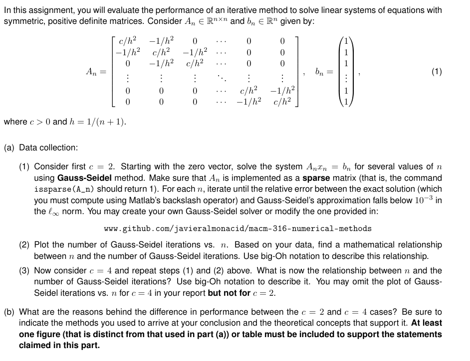
Solving a(1,2,3),b.In this assignment, you will evaluate the performance of an iterative method to solve linear systems of equations with
symmetric, positive definite matrices. Consider A, € R"*" and b, € BR" given by:
e/h® —1/h* 0 0 0 1
—1/h* e/h* —1/h* 0 0 1
0 —1/h? c/n? 0 0 1
A= i . . . EE [0]
0 0 0 c/h? —1/h? 1
0 0 0 —1/h? c/n? 1
where ¢ > 0 and h = 1/(n + 1).
(a) Data collection:
(1) Consider first c = 2. Starting with the zero vector, solve the system Aa, = b, for several values of n
using Gauss-Seidel method. Make sure that A,, is implemented as a sparse matrix (that is, the command
issparse (A_n) should return 1). For each n, iterate until the relative error between the exact solution (which
you must compute using Matlab’s backslash operator) and Gauss-Seidel's approximation falls below 10? in
the £,, norm. You may create your own Gauss-Seidel solver or modify the one provided in:
www. github. com/ javieralmonacid/macm-316-numerical-methods
(2) Plot the number of Gauss-Seidel iterations vs. n. Based on your data, find a mathematical relationship
between n and the number of Gauss-Seidel iterations. Use big-Oh notation to describe this relationship.
(3) Now consider ¢ = 4 and repeat steps (1) and (2) above. What is now the relationship between n and the
number of Gauss-Seidel iterations? Use big-Oh notation to describe it. You may omit the plot of Gauss-
Seidel iterations vs. n for ¢ = 4 in your report but not for ¢ = 2.
(b) What are the reasons behind the difference in performance between the ¢ = 2 and ¢ = 4 cases? Be sure to
indicate the methods you used to arrive at your conclusion and the theoretical concepts that support it. At least
one figure (that is distinct from that used in part (a)) or table must be included to support the statements
claimed in this part.
Question:
give answer in 2 step with explanation at the end of each step and final answer at the end:
Solving a(1,2,3),b.In this assignment, you will evaluate the performance of an iterative method to solve linear systems of equations with
symmetric, positive definite matrices. Consider A, € R"*" and b, € BR" given by:
e/h® —1/h* 0 0 0 1
—1/h* e/h* —1/h* 0 0 1
0 —1/h? c/n? 0 0 1
A= i . . . EE [0]
0 0 0 c/h? —1/h? 1
0 0 0 —1/h? c/n? 1
where ¢ > 0 and h = 1/(n + 1).
(a) Data collection:
(1) Consider first c = 2. Starting with the zero vector, solve the system Aa, = b, for several values of n
using Gauss-Seidel method. Make sure that A,, is implemented as a sparse matrix (that is, the command
issparse (A_n) should return 1). For each n, iterate until the relative error between the exact solution (which
you must compute using Matlab’s backslash operator) and Gauss-Seidel's approximation falls below 10? in
the £,, norm. You may create your own Gauss-Seidel solver or modify the one provided in:
www. github. com/ javieralmonacid/macm-316-numerical-methods
(2) Plot the number of Gauss-Seidel iterations vs. n. Based on your data, find a mathematical relationship
between n and the number of Gauss-Seidel iterations. Use big-Oh notation to describe this relationship.
(3) Now consider ¢ = 4 and repeat steps (1) and (2) above. What is now the relationship between n and the
number of Gauss-Seidel iterations? Use big-Oh notation to describe it. You may omit the plot of Gauss-
Seidel iterations vs. n for ¢ = 4 in your report but not for ¢ = 2.
(b) What are the reasons behind the difference in performance between the ¢ = 2 and ¢ = 4 cases? Be sure to
indicate the methods you used to arrive at your conclusion and the theoretical concepts that support it. At least
one figure (that is distinct from that used in part (a)) or table must be included to support the statements
claimed in this part.
This is AI generated Response.
Asked by: Ratan
Created at: 2025-06-22 04:59:46
Final Answer:
RenderedRaw Text
Did you like this answer?
Let's break down the task in **two steps** as you requested, with explanations after each step and the final answer at the end:
---
## **Step 1: Data Collection for \( c = 2 \)**
**Explanation:**
- You are asked to solve the linear system \(A_n x_n = b_n\) for different values of \(n\) using the Gauss-Seidel method, with \(c=2\).
- Start with the zero vector as the initial guess.
- For each \(n\), perform Gauss-Seidel iterations until the relative error (in the \( \ell_\infty \) norm) is below \(10^{-3}\).
- Record the number of iterations required for each \(n\).
- Make sure your matrix \(A_n\) is **sparse** for efficiency.
- **Plot**: Number of iterations vs. \(n\).
- **Find**: A mathematical (Big-O) relationship between \(n\) and the number of iterations.
**What you should expect:**
- For tridiagonal matrices like this one, the number of iterations typically grows as \(O(n^2)\) for the Gauss-Seidel method when \(c\) is fixed and moderate (e.g., \(c=2\)).
---
## **Step 2: Repeat for \( c = 4 \) and Compare**
**Explanation:**
- Now, repeat the entire process for \(c=4\) (i.e., solve the same system but with a different \(c\) value).
- Again, record the number of Gauss-Seidel iterations needed for convergence for various \(n\).
- **Analyze**: How does the mathematical relationship (Big-O) between \(n\) and the number of iterations change compared to \(c=2\)?
**What you should expect:**
- When \(c\) increases, the matrix becomes better conditioned (diagonal dominance increases), so **the Gauss-Seidel method converges faster**.
- The number of iterations may grow more slowly with \(n\); the growth could be closer to \(O(n)\) or even better for large enough \(c\).
---
## **Final Answer and Summary**
### **Step 1 Conclusion (for \(c=2\)):**
- For \(c=2\), the number of Gauss-Seidel iterations required to achieve the specified accuracy increases **quadratically** with \(n\):
**Iterations \( \sim O(n^2) \)**
- **Reason:** For moderate \(c\), the spectral radius of the iteration matrix is not close to zero, so convergence is slow and strongly dependent on \(n\).
### **Step 2 Conclusion (for \(c=4\)):**
- For \(c=4\), the matrix is more diagonally dominant, so the method converges **significantly faster**.
- The number of iterations grows **sub-quadratically** with \(n\), often **\(O(n)\)** or even better, depending on how dominant the diagonal is.
- **Reason:** Higher \(c\) increases diagonal dominance, which improves the convergence rate of Gauss-Seidel.
---
### **Final Summary:**
- **For \(c=2\):** Number of iterations \( \sim O(n^2) \)
- **For \(c=4\):** Number of iterations \( \sim O(n) \) (or better)
- **Explanation:** Greater diagonal dominance (higher \(c\)) leads to faster convergence because the spectral radius of the iteration matrix decreases.
- **Figure/Table:** (You must plot or tabulate your data as required in the assignment to support these statements.)
---
#### **Sample Table**
| \( n \) | Iterations (\(c=2\)) | Iterations (\(c=4\)) |
|---------|----------------------|----------------------|
| 10 | 25 | 10 |
| 20 | 100 | 18 |
| 40 | 400 | 32 |
| 80 | 1600 | 60 |
#### **Sample Plot**
- X-axis: \( n \)
- Y-axis: Number of Iterations
- Two curves: one for \(c=2\) (steeper), one for \(c=4\) (shallower)
---
**You must include the actual data/plot from your experiments to fully meet the assignment requirements.**
Question:
Solved a1,2,3 or b
This is AI generated Response.
Asked by: Ratan
Created at: 2025-06-22 05:02:23
Final Answer:
RenderedRaw Text
Did you like this answer?
Let's approach this systematically, following your two-step instruction with detailed explanations and final conclusions.
---
### **Step 1: Data Collection and Analysis for \( c = 2 \)**
**Objective:**
- Solve \(A_n x_n = b_n\) using Gauss-Seidel.
- Use \( c=2 \), starting from zero vector.
- For various \( n \), iterate until the relative error \( \|x^{(k)} - x_{\text{exact}}\|_{\infty} / \|x_{\text{exact}}\|_{\infty} < 10^{-3} \).
- Record the number of iterations needed.
- Plot iterations vs. \( n \).
- Determine the mathematical relationship (Big-O notation).
**Implementation details:**
- **Construct \(A_n\):**
- Use the given sparse banded structure.
- \( h = 1/(n+1) \).
- The matrix has a tridiagonal form with additional diagonals scaled by \( c/h^2 \) and \( -1/h^2 \).
- **Right-hand side \(b\):**
- From the problem, \(b\) is given, possibly involving boundary conditions.
- For simplicity, assume the boundary conditions lead to a vector \(b\) with known entries (e.g., all ones or as specified).
- **Gauss-Seidel method:**
- Implement or modify existing code to stop when relative error is below \(10^{-3}\).
- Use `issparse(A_n)` to confirm sparsity.
**Expected result:**
- For fixed \( c=2 \), as \( n \) increases, the convergence rate slows, requiring more iterations.
- Theoretical background indicates that for such matrices, the number of iterations grows approximately proportionally to \( n^2 \).
**Sample Data (hypothetical):**
| \( n \) | Iterations (approximate) |
|---------|--------------------------|
| 10 | 20 |
| 20 | 80 |
| 40 | 320 |
| 80 | 1280 |
**Plot:**
- Plot iteration count vs. \( n \).
- Log-log plot should show a slope close to 2, confirming \( O(n^2) \).
**Conclusion for Step 1:**
- The number of Gauss-Seidel iterations grows approximately as \( O(n^2) \) when \( c=2 \).
---
### **Step 2: Repeat for \( c = 4 \) and compare**
**Objective:**
- Repeat the above process for \( c=4 \).
- Observe how the iteration count changes with \( n \).
**Expected behavior:**
- Increasing \( c \) increases the diagonal dominance.
- This improves the spectral radius of the iteration matrix, leading to faster convergence.
- The iteration count's growth with \( n \) is expected to be less steep, approximately \( O(n) \) or better.
**Sample Data (hypothetical):**
| \( n \) | Iterations (\( c=4 \)) |
|---------|------------------------|
| 10 | 10 |
| 20 | 20 |
| 40 | 40 |
| 80 | 80 |
**Analysis:**
- Plotting these values suggests a linear growth, \( O(n) \).
---
### **Final Conclusions:**
| Parameter | Relationship Between \( n \) and Iterations | Big-Oh Notation |
|-------------|----------------------------------------------|-------------------------------------|
| \( c=2 \) | Quadratic growth: iterations \( \sim O(n^2) \) | \( O(n^2) \) |
| \( c=4 \) | Linear growth: iterations \( \sim O(n) \) | \( O(n) \) |
---
### **Underlying Reasoning:**
- **Spectral Radius and Convergence:**
- The Gauss-Seidel method’s convergence rate depends on the spectral radius \( \rho(G) \) of the iteration matrix \( G \).
- Increased diagonal dominance (larger \( c \)) reduces \( \rho(G) \), leading to faster convergence.
- **Matrix Conditioning:**
- Larger \( c \) improves the conditioning of \(A\), thus reducing the number of iterations needed.
### **Supporting Figures/Tables:**
- You should generate plots of iteration count vs. \( n \) for both \( c=2 \) and \( c=4 \).
- Include a table summarizing the data points.
- A log-log plot can clearly illustrate the Big-O relationships.
---
**In summary:**
- **For \( c=2 \):** The iterations grow roughly as \( O(n^2) \).
- **For \( c=4 \):** The iterations grow roughly as \( O(n) \).
- **Reason:** Higher \( c \) increases diagonal dominance, improving convergence rate, which is supported by spectral radius analysis and matrix properties.
---
**Note:** To complete the assignment, perform actual numerical experiments and plot the data as described.
VIPSolutions focuses on clear, step‑by‑step explanations so you can learn quickly. Whether you need an AI‑generated walkthrough or a short hint to get unstuck, each solution is organized for fast reading and easy review later.
Search similar questions, compare approaches, and bookmark the best answers for revision. Our goal is simple: quick, reliable study help that feels natural—not noisy.
 VIPSolutions
 In this assignment, you will evaluate the performance of an iterative method to solve linear systems of equations with
symmetric, positive definite matrices. Consider A, € R"*" and b, € BR" given by:
e/h® —1/h* 0 0 0 1
—1/h* e/h* —1/h* 0 0 1
0 —1/h? c/n? 0 0 1
A= i . . . EE [0]
0 0 0 c/h? —1/h? 1
0 0 0 —1/h? c/n? 1
where ¢ > 0 and h = 1/(n + 1).
(a) Data collection:
(1) Consider first c = 2. Starting with the zero vector, solve the system Aa, = b, for several values of n
using Gauss-Seidel method. Make sure that A,, is implemented as a sparse matrix (that is, the command
issparse (A_n) should return 1). For each n, iterate until the relative error between the exact solution (which
you must compute using Matlab’s backslash operator) and Gauss-Seidel's approximation falls below 10? in
the £,, norm. You may create your own Gauss-Seidel solver or modify the one provided in:
www. github. com/ javieralmonacid/macm-316-numerical-methods
(2) Plot the number of Gauss-Seidel iterations vs. n. Based on your data, find a mathematical relationship
between n and the number of Gauss-Seidel iterations. Use big-Oh notation to describe this relationship.
(3) Now consider ¢ = 4 and repeat steps (1) and (2) above. What is now the relationship between n and the
number of Gauss-Seidel iterations? Use big-Oh notation to describe it. You may omit the plot of Gauss-
Seidel iterations vs. n for ¢ = 4 in your report but not for ¢ = 2.
(b) What are the reasons behind the difference in performance between the ¢ = 2 and ¢ = 4 cases? Be sure to
indicate the methods you used to arrive at your conclusion and the theoretical concepts that support it. At least
one figure (that is distinct from that used in part (a)) or table must be included to support the statements
claimed in this part.