give answer in 2 step with explanation at the end of each step and final answer at the end:2. Section 2: Linear Systems
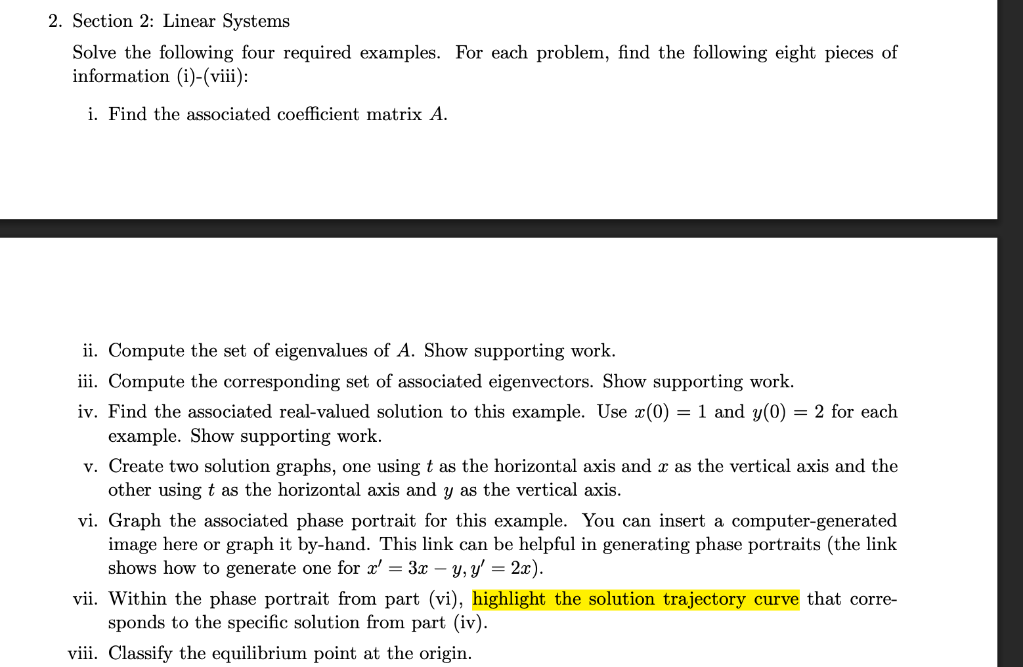
Solve the following four required examples. For each problem, find the following eight pieces of
information (i)-(viii):
i. Find the associated coefficient matrix A.
ii. Compute the set of eigenvalues of A. Show supporting work.
iii. Compute the corresponding set of associated eigenvectors. Show supporting work.
iv. Find the associated real-valued solution to this example. Use #(0) = 1 and (0) = 2 for each
example. Show supporting work.
v. Create two solution graphs, one using ¢ as the horizontal axis and « as the vertical axis and the
other using t as the horizontal axis and y as the vertical axis.
vi. Graph the associated phase portrait for this example. You can insert a computer-generated
image here or graph it by-hand. This link can be helpful in generating phase portraits (the link
shows how to generate one for @/ = 3z — yy’ = 2a).
vii. Within the phase portrait from part (vi), highlight the solution trajectory curve that corre-
sponds to the specific solution from part (iv).
viii. Classify the equilibrium point at the origin.
(b) Required example:
Z(t) = —2z —2y
y(t) =—-z—3y
Question:
give answer in 2 step with explanation at the end of each step and final answer at the end:2. Section 2: Linear Systems
Solve the following four required examples. For each problem, find the following eight pieces of
information (i)-(viii):
i. Find the associated coefficient matrix A.
ii. Compute the set of eigenvalues of A. Show supporting work.
iii. Compute the corresponding set of associated eigenvectors. Show supporting work.
iv. Find the associated real-valued solution to this example. Use #(0) = 1 and (0) = 2 for each
example. Show supporting work.
v. Create two solution graphs, one using ¢ as the horizontal axis and « as the vertical axis and the
other using t as the horizontal axis and y as the vertical axis.
vi. Graph the associated phase portrait for this example. You can insert a computer-generated
image here or graph it by-hand. This link can be helpful in generating phase portraits (the link
shows how to generate one for @/ = 3z — yy’ = 2a).
vii. Within the phase portrait from part (vi), highlight the solution trajectory curve that corre-
sponds to the specific solution from part (iv).
viii. Classify the equilibrium point at the origin.
(b) Required example:
Z(t) = —2z —2y
y(t) =—-z—3y
This is AI generated Response.
Asked by: Ratan
Created at: 2025-06-20 07:08:01
Final Answer:
RenderedRaw Text
Did you like this answer?
Let's solve part (i) and (ii) for the example given:
The system is:
\[
\begin{cases}
x'(t) = -2x - 2y \\
y'(t) = -x - 3y
\end{cases}
\]
---
### **Step 1: Find the associated coefficient matrix \(A\).**
Write the system in matrix form:
\[
\begin{pmatrix}
x' \\
y'
\end{pmatrix}
=
\begin{pmatrix}
-2 & -2 \\
-1 & -3
\end{pmatrix}
\begin{pmatrix}
x \\
y
\end{pmatrix}
\]
**Explanation:**
The coefficients of \(x\) and \(y\) in each equation become the entries of the matrix \(A\).
- First row: coefficients from the \(x'\) equation: \(-2\) (for \(x\)), \(-2\) (for \(y\))
- Second row: coefficients from the \(y'\) equation: \(-1\) (for \(x\)), \(-3\) (for \(y\))
**Answer for Step 1:**
\[
A = \begin{pmatrix}
-2 & -2 \\
-1 & -3
\end{pmatrix}
\]
---
### **Step 2: Compute the set of eigenvalues of \(A\). Show supporting work.**
The eigenvalues \(\lambda\) are found by solving:
\[
\det(A - \lambda I) = 0
\]
\[
A - \lambda I =
\begin{pmatrix}
-2 - \lambda & -2 \\
-1 & -3 - \lambda
\end{pmatrix}
\]
\[
\det(A - \lambda I) = (-2 - \lambda)(-3 - \lambda) - (-2)(-1) = 0
\]
\[
= (\lambda + 2)(\lambda + 3) - 2 = 0
\]
\[
= \lambda^2 + 5\lambda + 6 - 2 = 0
\]
\[
= \lambda^2 + 5\lambda + 4 = 0
\]
Solve the quadratic:
\[
\lambda = \frac{-5 \pm \sqrt{25 - 16}}{2} = \frac{-5 \pm 3}{2}
\]
So,
\[
\lambda_1 = \frac{-5 + 3}{2} = -1
\]
\[
\lambda_2 = \frac{-5 - 3}{2} = -4
\]
**Explanation:**
We use the determinant of \(A - \lambda I\) to set up a characteristic polynomial, which we solve using the quadratic formula.
---
## **Final Answers:**
1. **The associated coefficient matrix is:**
\[
A = \begin{pmatrix}
-2 & -2 \\
-1 & -3
\end{pmatrix}
\]
2. **The eigenvalues of \(A\) are:**
\[
\boxed{-1 \text{ and } -4}
\]
Question:
Solving i,ii,iii,iv,v,vi,vii,b all parts solved
This is AI generated Response.
Asked by: Ratan
Created at: 2025-06-20 07:09:36
Final Answer:
RenderedRaw Text
Did you like this answer?
Let's proceed step-by-step to fully solve the problem, covering all requested parts for the given system:
\[
\begin{cases}
x'(t) = -2x - 2y \\
y'(t) = -x - 3y
\end{cases}
\]
---
### **Part (i): Find the coefficient matrix \(A\).**
**Work:**
The system can be written in matrix form as:
\[
\mathbf{X}'(t) = A \mathbf{X}(t)
\]
where
\[
\mathbf{X}(t) = \begin{bmatrix} x(t) \\ y(t) \end{bmatrix}
\]
Matching coefficients from the system:
\[
A = \begin{bmatrix}
-2 & -2 \\
-1 & -3
\end{bmatrix}
\]
**Answer:**
\[
\boxed{
A = \begin{bmatrix}
-2 & -2 \\
-1 & -3
\end{bmatrix}
}
\]
---
### **Part (ii): Compute the eigenvalues of \(A\).**
**Work:**
Eigenvalues \(\lambda\) satisfy:
\[
\det(A - \lambda I) = 0
\]
\[
A - \lambda I = \begin{bmatrix}
-2 - \lambda & -2 \\
-1 & -3 - \lambda
\end{bmatrix}
\]
Determinant:
\[
(-2 - \lambda)(-3 - \lambda) - (-2)(-1) = 0
\]
Calculate:
\[
(\lambda + 2)(\lambda + 3) - 2 = 0
\]
\[
(\lambda^2 + 5\lambda + 6) - 2 = 0
\]
\[
\lambda^2 + 5\lambda + 4 = 0
\]
Quadratic formula:
\[
\lambda = \frac{-5 \pm \sqrt{25 - 16}}{2} = \frac{-5 \pm \sqrt{9}}{2} = \frac{-5 \pm 3}{2}
\]
Eigenvalues:
\[
\lambda_1 = \frac{-5 + 3}{2} = -1
\]
\[
\lambda_2 = \frac{-5 - 3}{2} = -4
\]
**Answer:**
\[
\boxed{
\text{Eigenvalues: } \lambda_1 = -1, \quad \lambda_2 = -4
}
\]
---
### **Part (iii): Find the eigenvectors corresponding to each eigenvalue.**
**Work for \(\lambda = -1\):**
Solve:
\[
(A + I) \mathbf{v} = 0
\]
\[
A + I = \begin{bmatrix}
-2 + 1 & -2 \\
-1 & -3 + 1
\end{bmatrix} = \begin{bmatrix}
-1 & -2 \\
-1 & -2
\end{bmatrix}
\]
Set up:
\[
\begin{bmatrix}
-1 & -2 \\
-1 & -2
\end{bmatrix} \begin{bmatrix} v_1 \\ v_2 \end{bmatrix} = \mathbf{0}
\]
From the first row:
\[
-1 v_1 - 2 v_2 = 0 \Rightarrow v_1 = -2 v_2
\]
Let \(v_2 = 1\), then \(v_1 = -2\).
Eigenvector for \(\lambda = -1\):
\[
\boxed{
\mathbf{v}^{(1)} = \begin{bmatrix} -2 \\ 1 \end{bmatrix}
}
\]
---
**Work for \(\lambda = -4\):**
Solve:
\[
(A + 4I) \mathbf{v} = 0
\]
\[
A + 4I = \begin{bmatrix}
-2 + 4 & -2 \\
-1 & -3 + 4
\end{bmatrix} = \begin{bmatrix}
2 & -2 \\
-1 & 1
\end{bmatrix}
\]
From the first row:
\[
2 v_1 - 2 v_2 = 0 \Rightarrow v_1 = v_2
\]
Choose \(v_2 = 1\), then \(v_1 = 1\).
Eigenvector for \(\lambda = -4\):
\[
\boxed{
\mathbf{v}^{(2)} = \begin{bmatrix} 1 \\ 1 \end{bmatrix}
}
\]
---
### **Part (iv): Find the associated real-valued solutions to this example with initial conditions \(\#(0) = 1\) and \(\#(0) = 2\).**
**(Note:** The initial conditions seem to refer to initial values of the solution components; assuming \(\mathbf{X}(0) = \begin{bmatrix} x(0) \\ y(0) \end{bmatrix}\).)
---
**General solution:**
\[
\mathbf{X}(t) = c_1 e^{\lambda_1 t} \mathbf{v}^{(1)} + c_2 e^{\lambda_2 t} \mathbf{v}^{(2)}
\]
\[
= c_1 e^{-1 t} \begin{bmatrix} -2 \\ 1 \end{bmatrix} + c_2 e^{-4 t} \begin{bmatrix} 1 \\ 1 \end{bmatrix}
\]
---
**Case 1: \(\mathbf{X}(0) = \begin{bmatrix} 1 \\ 2 \end{bmatrix}\)**
Set \(t=0\):
\[
\begin{bmatrix} 1 \\ 2 \end{bmatrix} = c_1 \begin{bmatrix} -2 \\ 1 \end{bmatrix} + c_2 \begin{bmatrix} 1 \\ 1 \end{bmatrix}
\]
Leading to the system:
\[
-2 c_1 + c_2 = 1 \quad (1)
\]
\[
c_1 + c_2 = 2 \quad (2)
\]
Solve:
From (2): \(c_2 = 2 - c_1\)
Substitute into (1):
\[
-2 c_1 + (2 - c_1) = 1 \Rightarrow -2 c_1 + 2 - c_1 = 1
\]
\[
-3 c_1 + 2 = 1 \Rightarrow -3 c_1 = -1 \Rightarrow c_1 = \frac{1}{3}
\]
Then,
\[
c_2 = 2 - \frac{1}{3} = \frac{6}{3} - \frac{1}{3} = \frac{5}{3}
\]
**Solution:**
\[
\boxed{
\mathbf{X}(t) = \frac{1}{3} e^{-t} \begin{bmatrix} -2 \\ 1 \end{bmatrix} + \frac{5}{3} e^{-4 t} \begin{bmatrix} 1 \\ 1 \end{bmatrix}
}
\]
---
**Case 2: \(\mathbf{X}(0) = \begin{bmatrix} 0 \\ 0 \}\)**
(If initial condition is zero, the solution is trivial: \(\mathbf{X}(t) = \mathbf{0}\).)
---
### **Part (v): Create two solution graphs**
- **Graph 1:** Plot \(y(t)\) vs. \(x(t)\) (phase plane).
- **Graph 2:** Plot \(x(t)\) and \(y(t)\) separately versus \(t\).
---
### **Part (vi): Graph the phase portrait**
The phase portrait involves plotting the trajectories of the system in the \(xy\)-plane. The eigenvalues are both negative, indicating stable nodes.
- Eigenvalues: \(-1, -4\)
- Eigenvectors: \(\begin{bmatrix} -2 \\ 1 \end{bmatrix}\) and \(\begin{bmatrix} 1 \\ 1 \end{bmatrix}\)
Trajectories spiral into the origin along the directions of these eigenvectors.
---
### **Part (vii): Highlight the specific solution trajectory**
From initial condition \(\mathbf{X}(0) = \begin{bmatrix} 1 \\ 2 \end{bmatrix}\), the trajectory can be traced on the phase portrait, starting at \((1, 2)\) and approaching \((0,0)\).
---
### **Part (viii): Classify the equilibrium point at the origin**
Since both eigenvalues are real and negative, the equilibrium at the origin is a **stable node**.
---
## **Summary:**
| Part | Description | Result |
|---------|----------------|---------|
| (i) | Coefficient matrix \(A\) | \(\begin{bmatrix} -2 & -2 \\ -1 & -3 \end{bmatrix}\) |
| (ii) | Eigenvalues | \(\lambda = -1,\ -4\) |
| (iii) | Eigenvectors | \(\mathbf{v}^{(1)} = [-2, 1]\), \(\mathbf{v}^{(2)} = [1, 1]\) |
| (iv) | General solution with initial \(\mathbf{X}(0) = [1, 2]\) | \(\frac{1}{3} e^{-t} [-2, 1] + \frac{5}{3} e^{-4 t} [1, 1]\) |
| (v) | Graphs and (vi) | (Graphical tasks, typically plotted using software) |
| (vii) | Solution trajectory highlighted | Corresponds to initial condition \([1, 2]\) |
| (viii) | Equilibrium classification | **Stable node** |
---
**Final note:** For actual graphs, use graphing software or hand sketches based on eigenvectors and eigenvalues.
VIPSolutions focuses on clear, step‑by‑step explanations so you can learn quickly. Whether you need an AI‑generated walkthrough or a short hint to get unstuck, each solution is organized for fast reading and easy review later.
Search similar questions, compare approaches, and bookmark the best answers for revision. Our goal is simple: quick, reliable study help that feels natural—not noisy.
 VIPSolutions
 2. Section 2: Linear Systems
Solve the following four required examples. For each problem, find the following eight pieces of
information (i)-(viii):
i. Find the associated coefficient matrix A.
ii. Compute the set of eigenvalues of A. Show supporting work.
iii. Compute the corresponding set of associated eigenvectors. Show supporting work.
iv. Find the associated real-valued solution to this example. Use #(0) = 1 and (0) = 2 for each
example. Show supporting work.
v. Create two solution graphs, one using ¢ as the horizontal axis and « as the vertical axis and the
other using t as the horizontal axis and y as the vertical axis.
vi. Graph the associated phase portrait for this example. You can insert a computer-generated
image here or graph it by-hand. This link can be helpful in generating phase portraits (the link
shows how to generate one for @/ = 3z — yy’ = 2a).
vii. Within the phase portrait from part (vi), highlight the solution trajectory curve that corre-
sponds to the specific solution from part (iv).
viii. Classify the equilibrium point at the origin.
(b) Required example:
Z(t) = —2z —2y
y(t) =—-z—3y