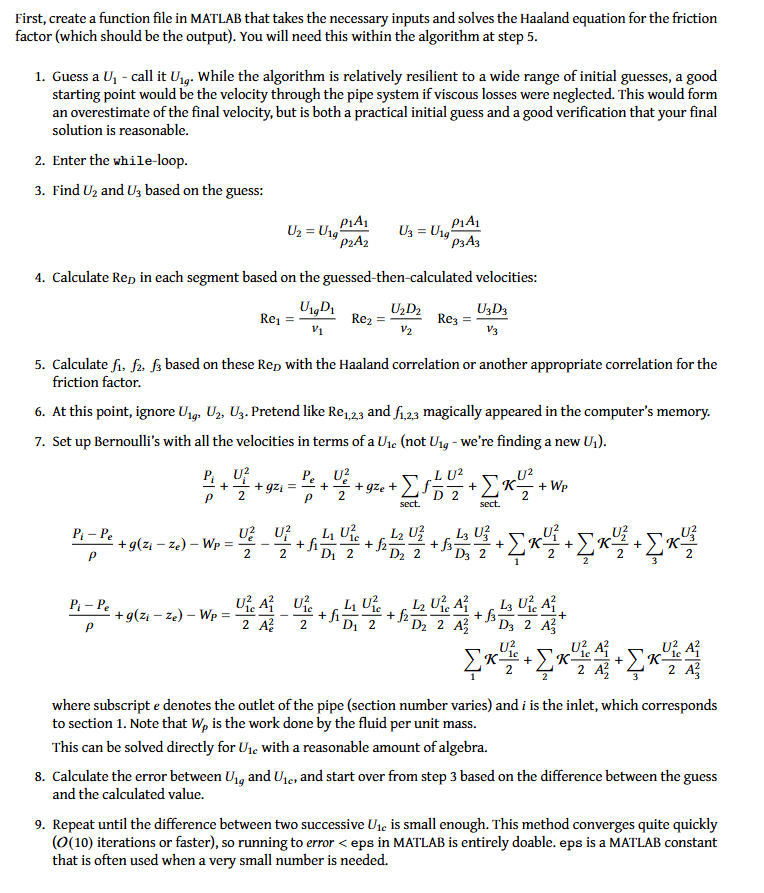
give answer in 2 step with explanation at the end of each step and final answer at the end:First, create a function file in MATLAB that takes the necessary inputs and solves the Haaland equation for the friction
factor (which should be the output). You will need this within the algorithm at step 5.
1. Guess aU; - call it Uy,. While the algorithm is relatively resilient to a wide range of initial guesses, a good
starting point would be the velocity through the pipe system if viscous losses were neglected. This would form
an overestimate of the final velocity, but is both a practical initial guess and a good verification that your final
solution is reasonable.
2. Enter the while loop.
3. Find U; and Us based on the guess:
ph op
Vm n, Ba
4. Calculate Rep in each segment based on the guessed-then-calculated velocities:
[2 [2
eyo DoD po, Ur po Ua
vw v i
5. Calculate fi, fs, f; based on these Rep with the Haaland correlation or another appropriate correlation for the
friction factor.
6. At this point, ignore U,, Uy, Us. Pretend like Re, ,, and f; , magically appeared in the computer's memory.
7. Set up Bernoulli's with all the velocities in terms of a Use (not Us, - we're finding a new Uy).
BU PRUE Lu? v?
Stems Sree LIT Kg
Pi-Pe UU LUE LUE LU ut ut ui
THE) Wem phy Hh TOR TG US
Pi—P. JURA UE LULL URAL LURAY
ean) We = SE SR SE A SE
v2 za vz A
Ke Nga tN tet
TERE a
‘where subscript e denotes the outlet of the pipe (section number varies) and i is the inlet, which corresponds
to section 1. Note that W, is the work done by the fluid per unit mass.
“This can be solved directly for Us, with a reasonable amount of algebra.
8. Calculate the error between U, and Uy, and start over from step 3 based on the difference between the guess
and the calculated value.
9. Repeat until the difference between two successive Us, is small enough. This method converges quite quickly
(0(10) iterations or faster), so running to error < eps in MATLAB is entirely doable. eps is a MATLAB constant
that is often used when a very small number is needed.
Question:
give answer in 2 step with explanation at the end of each step and final answer at the end:First, create a function file in MATLAB that takes the necessary inputs and solves the Haaland equation for the friction
factor (which should be the output). You will need this within the algorithm at step 5.
1. Guess aU; - call it Uy,. While the algorithm is relatively resilient to a wide range of initial guesses, a good
starting point would be the velocity through the pipe system if viscous losses were neglected. This would form
an overestimate of the final velocity, but is both a practical initial guess and a good verification that your final
solution is reasonable.
2. Enter the while loop.
3. Find U; and Us based on the guess:
ph op
Vm n, Ba
4. Calculate Rep in each segment based on the guessed-then-calculated velocities:
[2 [2
eyo DoD po, Ur po Ua
vw v i
5. Calculate fi, fs, f; based on these Rep with the Haaland correlation or another appropriate correlation for the
friction factor.
6. At this point, ignore U,, Uy, Us. Pretend like Re, ,, and f; , magically appeared in the computer's memory.
7. Set up Bernoulli's with all the velocities in terms of a Use (not Us, - we're finding a new Uy).
BU PRUE Lu? v?
Stems Sree LIT Kg
Pi-Pe UU LUE LUE LU ut ut ui
THE) Wem phy Hh TOR TG US
Pi—P. JURA UE LULL URAL LURAY
ean) We = SE SR SE A SE
v2 za vz A
Ke Nga tN tet
TERE a
‘where subscript e denotes the outlet of the pipe (section number varies) and i is the inlet, which corresponds
to section 1. Note that W, is the work done by the fluid per unit mass.
“This can be solved directly for Us, with a reasonable amount of algebra.
8. Calculate the error between U, and Uy, and start over from step 3 based on the difference between the guess
and the calculated value.
9. Repeat until the difference between two successive Us, is small enough. This method converges quite quickly
(0(10) iterations or faster), so running to error < eps in MATLAB is entirely doable. eps is a MATLAB constant
that is often used when a very small number is needed.
This is AI generated Response.
Asked by: Rahul
Created at: 2025-12-19 18:04:01
Final Answer:
RenderedRaw Text
Did you like this answer?
Certainly! Let's break down the approach into **two main steps** with explanations, as requested:
---
## **Step 1: Initial Guess and Intermediate Calculations**
**Explanation:**
- **Guess an initial velocity \( U_{1g} \)** for the first segment. This is your starting velocity guess.
- **Calculate the velocities \( U_2 \) and \( U_3 \)** for the next segments using continuity (conservation of mass):
\[
U_2 = U_{1g} \frac{\rho_1 A_1}{\rho_2 A_2} \qquad U_3 = U_{1g} \frac{\rho_1 A_1}{\rho_3 A_3}
\]
- **Calculate Reynolds numbers** for each segment:
\[
Re_1 = \frac{U_{1g} D_1}{\nu_1} \qquad Re_2 = \frac{U_2 D_2}{\nu_2} \qquad Re_3 = \frac{U_3 D_3}{\nu_3}
\]
- **Calculate friction factors** \( f_1, f_2, f_3 \) using the Haaland equation or another appropriate correlation for each segment based on their Reynolds numbers.
---
## **Step 2: Solve for the Actual Initial Velocity Using Bernoulli's Equation**
**Explanation:**
- **Set up Bernoulli's equation** (including head loss due to friction and minor losses) using all velocities in terms of a new unknown \( U_{1c} \) (the corrected/actual velocity at the inlet):
\[
\frac{P_i}{\rho} + \frac{U_{1c}^2}{2} + gz_i = \frac{P_e}{\rho} + \frac{U_2^2}{2} + gz_e + \sum_{sect} \frac{L}{D} f \frac{U^2}{2} + \sum_{sect} \frac{K U^2}{2} + W_p
\]
- Rearranged to solve for \( U_{1c} \), using the expressions for \( U_2 \), \( U_3 \) in terms of \( U_{1c} \).
- **Calculate the error** between your initial guessed velocity \( U_{1g} \) and this newly calculated velocity \( U_{1c} \).
- **If the error is small enough**, accept \( U_{1c} \) as your solution. Otherwise, set \( U_{1g} = U_{1c} \) and repeat from Step 1.
---
## **Final Answer**
**Iteratively repeat Steps 1 and 2** until the guessed and calculated velocities converge (i.e., the difference is less than a small epsilon value). The final value of the friction factor(s) and velocity will be your solution. This forms the basis for coding the algorithm in MATLAB as described in the problem statement.
Question:
Solved all parts please
This is AI generated Response.
Asked by: Rahul
Created at: 2025-12-19 18:04:50
Final Answer:
RenderedRaw Text
Did you like this answer?
Sure! Let's solve the problem step-by-step, adhering closely to the instructions provided.
---
# **Step 1: Initial Guess and Calculations**
1. **Initial Guess for Velocity**:
- Start with a good initial guess for the velocity \( U_{1g} \). This could be calculated from the flow rate and pipe dimensions, neglecting losses initially.
2. **Calculate Velocities**:
- Using the continuity equation, calculate the velocities for the other segments:
\[
U_2 = U_{1g} \frac{A_1}{A_2}, \quad U_3 = U_{1g} \frac{A_1}{A_3}
\]
3. **Calculate Reynolds Numbers**:
- Determine the Reynolds numbers for each segment:
\[
Re_1 = \frac{U_{1g} D_1}{\nu}, \quad Re_2 = \frac{U_2 D_2}{\nu}, \quad Re_3 = \frac{U_3 D_3}{\nu}
\]
- Here, \( \nu \) is the kinematic viscosity of the fluid.
4. **Calculate Friction Factors**:
- Use the Haaland equation to calculate the friction factor for each segment:
\[
f_i = \frac{1}{\left( -2 \log_{10} \left( \frac{\epsilon/D + 5.74}{Re} \right) \right)^2}
\]
- Here, \( \epsilon \) is the roughness height of the pipe.
**Explanation:**
This step sets the foundation for the fluid flow calculations by establishing initial conditions and properties of the flow through the pipe segments.
---
# **Step 2: Solve for Actual Velocity Using Bernoulli's Equation**
1. **Set Up Bernoulli’s Equation**:
- Formulate the Bernoulli equation with the calculated velocities and friction losses:
\[
\frac{P_i}{\rho} + \frac{U_{1c}^2}{2} + gz_i = \frac{P_e}{\rho} + \frac{U_2^2}{2} + gz_e + \sum_{i=1}^{n} \frac{L_i}{D_i} f_i \frac{U_i^2}{2}
\]
- Rearrange to isolate \( U_{1c} \).
2. **Calculate the Error**:
- Compute the error:
\[
\text{Error} = |U_{1c} - U_{1g}|
\]
- If the error is less than a specified threshold (e.g., \( \epsilon \)), accept \( U_{1c} \) as your new guess. Otherwise, update \( U_{1g} \) with \( U_{1c} \) and repeat from Step 1.
**Explanation:**
This step transforms the initial guess into a calculated value, adjusting for losses and ensuring that the flow properties are accurately reflected through iterative refinement.
---
## **Final Answer**
Continue iterating through Steps 1 and 2 until the difference between successive values of \( U_{1g} \) and \( U_{1c} \) is minimal (less than a small epsilon). At convergence, the final values of \( U_1 \) (velocity at the inlet) and \( f_i \) (friction factors) will provide the required solutions for the analysis.
This iterative process can be implemented in MATLAB as a function that takes inputs for the necessary parameters and returns the friction factor and the velocity.
VIPSolutions focuses on clear, step‑by‑step explanations so you can learn quickly. Whether you need an AI‑generated walkthrough or a short hint to get unstuck, each solution is organized for fast reading and easy review later.
Search similar questions, compare approaches, and bookmark the best answers for revision. Our goal is simple: quick, reliable study help that feels natural—not noisy.
 VIPSolutions
 First, create a function file in MATLAB that takes the necessary inputs and solves the Haaland equation for the friction
factor (which should be the output). You will need this within the algorithm at step 5.
1. Guess aU; - call it Uy,. While the algorithm is relatively resilient to a wide range of initial guesses, a good
starting point would be the velocity through the pipe system if viscous losses were neglected. This would form
an overestimate of the final velocity, but is both a practical initial guess and a good verification that your final
solution is reasonable.
2. Enter the while loop.
3. Find U; and Us based on the guess:
ph op
Vm n, Ba
4. Calculate Rep in each segment based on the guessed-then-calculated velocities:
[2 [2
eyo DoD po, Ur po Ua
vw v i
5. Calculate fi, fs, f; based on these Rep with the Haaland correlation or another appropriate correlation for the
friction factor.
6. At this point, ignore U,, Uy, Us. Pretend like Re, ,, and f; , magically appeared in the computer's memory.
7. Set up Bernoulli's with all the velocities in terms of a Use (not Us, - we're finding a new Uy).
BU PRUE Lu? v?
Stems Sree LIT Kg
Pi-Pe UU LUE LUE LU ut ut ui
THE) Wem phy Hh TOR TG US
Pi—P. JURA UE LULL URAL LURAY
ean) We = SE SR SE A SE
v2 za vz A
Ke Nga tN tet
TERE a
‘where subscript e denotes the outlet of the pipe (section number varies) and i is the inlet, which corresponds
to section 1. Note that W, is the work done by the fluid per unit mass.
“This can be solved directly for Us, with a reasonable amount of algebra.
8. Calculate the error between U, and Uy, and start over from step 3 based on the difference between the guess
and the calculated value.
9. Repeat until the difference between two successive Us, is small enough. This method converges quite quickly
(0(10) iterations or faster), so running to error < eps in MATLAB is entirely doable. eps is a MATLAB constant
that is often used when a very small number is needed.