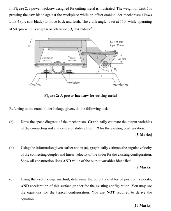
## Step-by-Step Solution --- ### **Step 1: Space Diagram & Output Variables (Part)** ####Explanation** -Space Diagram** Draw the crank-slider mechanism as shown in Figure 2, labeling all links and joints. - **O₂**: Fixed pivot for the crank (Link 2). - **A**: Crank-connecting rod joint. - **B**: Slider end (centre of saw blade). - **Link 2**: Crank (O₂A, length L₂ = 75 mm, angle θ₂ = 110°). - **Link 3**: Connecting rod (AB, length L₃ = 170 mm). - **Link 4**: Slider (point B, offset 45 mm from OA line). - **Graphical Estimation**: 1. **Draw O₂A** at 110° from the horizontal, length 75 mm. 2. **Draw a circle** with radius L₃ = 170 mm from point A. 3. **Draw the slider path** as a straight line, offset 45 mm vertically from O₂. 4. **Intersection** of the circle and slider path gives point B. - **Output Variables**: - **Position of connecting rod**: Line AB. - **Centre of slider at B**: Coordinates of B from the diagram. #### **Explanation End of Step 1** By constructing the geometry, you find the instantaneous positions of all points, particularly the connecting rod's orientation and the slider's centre. This sets up all kinematic relationships for subsequent velocity/acceleration analysis. --- ### **Step 2: Velocities & Vector-Loop Analysis (Parts b & c)** #### **Explanation** - **Given**: - Crank angular velocity, ω₂ = 2π × 50 / 60 ≈ 5.24 rad/s - Crank angular acceleration, α₂ = 4 rad/s² - θ₂ = 110° #### **(b) Velocity Analysis, Graphically** 1. **Draw the velocity diagram**: - Start with the velocity of A: \( V_A = ω_2 \times L_2 \) - Draw VA perpendicular to O₂A (since crank rotates). - From A, draw the velocity of B (VB) along the slider path (horizontal). - Draw the relative velocity of B with respect to A (V_{B/A}), perpendicular to AB. - The intersection locates VB and V_{B/A}. 2. **Find**: - **Angular velocity of connecting rod**: \( ω_3 = \frac{V_{B/A}}{L_3} \) - **Linear velocity of slider (B)**: \( V_B \) (measured from diagram). #### **(c) Vector-Loop Method (Position, Velocity, Acceleration)** - **Loop-closure equation** for this mechanism (all vectors as complex numbers): \[ \vec{r}_2 + \vec{r}_3 = \vec{r}_4 \] Where: - \( \vec{r}_2 = L_2 (\cos θ_2 \hat{i} + \sin θ_2 \hat{j}) \) - \( \vec{r}_3 = L_3 (\cos θ_3 \hat{i} + \sin θ_3 \hat{j}) \) - \( \vec{r}_4 \): Horizontal displacement of B, offset by 45 mm vertically - **Velocity equations (by differentiation):** \[ \omega_2 \vec{e}_{2\perp} L_2 + \omega_3 \vec{e}_{3\perp} L_3 = V_B \hat{i} \] - Solve for \( ω_3 \) and \( V_B \) (slider velocity). - **Acceleration equations (by differentiation):** \[ α_2 \vec{e}_{2\perp} L_2 - ω_2^2 \vec{r}_2 + α_3 \vec{e}_{3\perp} L_3 - ω_3^2 \vec{r}_3 = a_B \hat{i} \] - Solve for \( α_3 \) and \( a_B \) (slider acceleration). #### **Explanation End of Step 2** The vector-loop method yields the **exact positions**, **velocities**, and **accelerations** for all links at the given instant, using the crank angle and rates as input. --- ## **Final Answer** 1. **Space diagram** enables the clear identification of all points, link lengths, and their positions for the mechanism at the given crank angle, providing a geometric foundation for kinematic analysis. 2. **Velocity and acceleration analysis** (both graphically and analytically via the vector-loop method) allows for the determination of output variables (positions, velocities, and accelerations) for all links, especially the connecting rod and slider, at the specified configuration. **By following these two steps, you can fully analyze the kinematics of the power hacksaw mechanism for the given configuration.**

# Kinematic Analysis of a Power Hacksaw Mechanism ## Step-by-Step Solution --- ### **Step 1: Space Diagram & Output Variables** #### **Explanation** - **Space Diagram**: Draw the crank-slider mechanism as per Figure 2. - **O₂**: Fixed pivot for crank (Link 2). - **A**: Crank-connecting rod joint. - **B**: Slider end (centre of saw blade). - **Link 2**: Crank (O₂A, length \( L_2 = 75 \) mm, angle \( θ_2 = 110° \)). - **Link 3**: Connecting rod (AB, length \( L_3 = 170 \) mm). - **Link 4**: Slider (point B, offset 45 mm from OA line). - **Graphical Estimation**: 1. **Draw O₂A** at \( 110° \) from the horizontal, length \( 75 \) mm. 2. **Draw a circle** with radius \( L_3 = 170 \) mm from point A. 3. **Draw the slider path** as a straight line, offset 45 mm vertically from O₂. 4. **Find intersection** of the circle and slider path to locate point B. - **Output Variables**: - **Position of connecting rod**: Line AB. - **Coordinates of slider at B**: Derived from the intersection point. #### **Explanation End of Step 1** This step establishes the geometric layout of the system, which is critical for analyzing kinematic relationships among the links. --- ### **Step 2: Velocities & Vector-Loop Analysis** #### **Explanation** - **Given Data**: - Crank angular velocity, \( ω_2 = \frac{2\pi \times 50}{60} \approx 5.24 \, \text{rad/s} \) - Crank angular acceleration, \( α_2 = 4 \, \text{rad/s}^2 \) - Crank angle, \( θ_2 = 110° \) #### **(b) Velocity Analysis (Graphically)** 1. **Velocity Diagram**: - Compute velocity of A: \[ V_A = ω_2 \times L_2 = 5.24 \times 0.075\, \text{m} \approx 0.393\, \text{m/s} \] - Draw \( V_A \) perpendicular to O₂A. - From A, draw \( V_B \) along the slider path (horizontal). - Draw relative velocity \( V_{B/A} \) perpendicular to AB. - Intersection of \( V_B \) and \( V_{B/A} \) locates \( V_B \). 2. **Find**: - **Angular velocity of connecting rod**: \[ ω_3 = \frac{V_{B/A}}{L_3} \] - **Linear velocity of slider (B)**: Measured from the diagram. #### **(c) Vector-Loop Method (Position, Velocity, Acceleration)** - **Loop-closure equation**: \[ \vec{r}_2 + \vec{r}_3 = \vec{r}_4 \] Where: - \( \vec{r}_2 = L_2 (\cos θ_2 \hat{i} + \sin θ_2 \hat{j}) \) - \( \vec{r}_3 = L_3 (\cos θ_3 \hat{i} + \sin θ_3 \hat{j}) \) - \( \vec{r}_4 \): Horizontal displacement of B, offset by 45 mm. - **Velocity equations (differentiation)**: \[ ω_2 \vec{e}_{2\perp} L_2 + ω_3 \vec{e}_{3\perp} L_3 = V_B \hat{i} \] - Solve for \( ω_3 \) and \( V_B \). - **Acceleration equations (differentiation)**: \[ α_2 \vec{e}_{2\perp} L_2 - ω_2^2 \vec{r}_2 + α_3 \vec{e}_{3\perp} L_3 - ω_3^2 \vec{r}_3 = a_B \hat{i} \] - Solve for \( α_3 \) and \( a_B \). #### **Explanation End of Step 2** The vector-loop method provides detailed kinematic information, including positions, velocities, and accelerations for all links, particularly the connecting rod and slider, at the specified crank configuration. --- ## **Final Answer** 1. **Space Diagram**: Clearly identifies all link positions and orientations for the mechanism at the crank angle of 110°. 2. **Velocity and Acceleration Analysis**: Through graphical and vector-loop methods, the analysis yields precise values for the velocities and accelerations of the connecting rod and slider, essential for understanding the mechanism's kinematics.