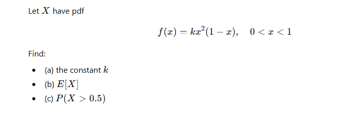
FIRST WRITE GIVENINFORMATION THENWHAT HAVE TO FIND AND THEN DEFINATION ORCONCEPT USED AND THEN STEP BY STEPSOLUTION WITHOUT MENTIONING STEP NUMBER AND AT LAST WRITE FINALANSWERS ONLY AS SUMMARY . ALSO MAKE SOLUTION WELL STRUCTUREDLet X have pdf
fl@)=ka*(l-z), 0
Question:
FIRST WRITE GIVENINFORMATION THENWHAT HAVE TO FIND AND THEN DEFINATION ORCONCEPT USED AND THEN STEP BY STEPSOLUTION WITHOUT MENTIONING STEP NUMBER AND AT LAST WRITE FINALANSWERS ONLY AS SUMMARY . ALSO MAKE SOLUTION WELL STRUCTUREDLet X have pdf
fl@)=ka*(l-z), 0
This is AI generated Response.
Asked by: nayan
Created at: 2026-02-12 20:57:02
Final Answer:
RenderedRaw Text
Did you like this answer?
# Given Information
- The random variable \( X \) has the probability density function (pdf):
\[
f(x) = kx^2(1-x), \quad < x < 1
\]
# What Have to Find
- (a) The constant \( k \)
- (b) The expected value \( E[X] \)
- (c) The probability \( P(X > .5) \)
# Definition or Concept Used
- The total probability for a continuous random variable must be 1: \(\int_{-\infty}^{\infty} f(x)\,dx = 1\).
- Expected value: \(E[X] = \int_{-\infty}^{\infty} x f(x)\,dx\)
- Probability over an interval: \(P(X > a) = \int_{a}^{\infty} f(x)\,dx\)
# Step-by-Step Solution
**(a) Finding the constant \( k \):**
Set the total probability to 1:
\[
\int_^1 kx^2(1-x)\,dx = 1
\]
\[
k \int_^1 (x^2 - x^3)\,dx = 1
\]
\[
k \left[ \frac{x^3}{3} - \frac{x^4}{4} \right]_^1 = 1
\]
\[
k \left( \frac{1}{3} - \frac{1}{4} \right) = 1
\]
\[
k \left( \frac{4-3}{12} \right) = 1
\]
\[
k \cdot \frac{1}{12} = 1
\]
\[
k = 12
\]
**(b) Finding the expected value \( E[X] \):**
\[
E[X] = \int_^1 x f(x)\,dx = \int_^1 x \cdot 12x^2(1-x)\,dx
\]
\[
= 12 \int_^1 x^3(1-x)\,dx
\]
\[
= 12 \int_^1 (x^3 - x^4)\,dx
\]
\[
= 12 \left[ \frac{x^4}{4} - \frac{x^5}{5} \right]_^1
\]
\[
= 12 \left( \frac{1}{4} - \frac{1}{5} \right)
\]
\[
= 12 \cdot \frac{5-4}{20}
\]
\[
= 12 \cdot \frac{1}{20}
\]
\[
= \frac{12}{20} = \frac{3}{5}
\]
**(c) Finding \( P(X > .5) \):**
\[
P(X > .5) = \int_{.5}^1 12x^2(1-x)\,dx
\]
\[
= 12 \int_{.5}^1 (x^2 - x^3)\,dx
\]
\[
= 12 \left[ \frac{x^3}{3} - \frac{x^4}{4} \right]_{.5}^1
\]
\[
= 12 \left( \left[ \frac{1}{3} - \frac{1}{4} \right] - \left[ \frac{(.5)^3}{3} - \frac{(.5)^4}{4} \right] \right)
\]
\[
= 12 \left( \frac{1}{12} - \left[ \frac{.125}{3} - \frac{.0625}{4} \right] \right)
\]
\[
= 12 \left( \frac{1}{12} - \left[ .04167 - .015625 \right] \right)
\]
\[
= 12 \left( \frac{1}{12} - .026045 \right)
\]
\[
= 12 \left( .08333 - .026045 \right)
\]
\[
= 12 \times .057285
\]
\[
= .68742
\]
# Summary
- \( k = 12 \)
- \( E[X] = \frac{3}{5} \)
- \( P(X > .5) \approx .687 \)
Question:
make solutino well structured
This is AI generated Response.
Asked by: nayan
Created at: 2026-02-12 20:59:10
Final Answer:
RenderedRaw Text
Did you like this answer?
# Given Information
- The random variable \( X \) has the probability density function (pdf):
\[
f(x) = kx^2(1-x), \quad 0 < x < 1
\]
# What We Need to Find
- (a) The constant \( k \)
- (b) The expected value \( E[X] \)
- (c) The probability \( P(X > 0.5) \)
# Definitions or Concepts Used
- **Total Probability**: The total probability for a continuous random variable must equal 1:
\[
\int_{-\infty}^{\infty} f(x)\,dx = 1
\]
- **Expected Value**: The expected value is calculated as:
\[
E[X] = \int_{-\infty}^{\infty} x f(x)\,dx
\]
- **Probability Over an Interval**: The probability that \( X \) exceeds a certain value \( a \) is given by:
\[
P(X > a) = \int_{a}^{\infty} f(x)\,dx
\]
# Step-by-Step Solution
**Finding the Constant \( k \)**
Set the total probability to 1:
\[
\int_0^1 kx^2(1-x)\,dx = 1
\]
This simplifies to:
\[
k \int_0^1 (x^2 - x^3)\,dx = 1
\]
Calculating the integral:
\[
k \left[ \frac{x^3}{3} - \frac{x^4}{4} \right]_0^1 = 1
\]
\[
k \left( \frac{1}{3} - \frac{1}{4} \right) = 1
\]
\[
k \cdot \frac{1}{12} = 1 \quad \Rightarrow \quad k = 12
\]
**Finding the Expected Value \( E[X] \)**
Calculate \( E[X] \):
\[
E[X] = \int_0^1 x f(x)\,dx = \int_0^1 x \cdot 12x^2(1-x)\,dx
\]
This becomes:
\[
= 12 \int_0^1 (x^3 - x^4)\,dx
\]
Calculating the integral:
\[
= 12 \left[ \frac{x^4}{4} - \frac{x^5}{5} \right]_0^1
\]
\[
= 12 \left( \frac{1}{4} - \frac{1}{5} \right) = 12 \cdot \frac{1}{20} = \frac{12}{20} = \frac{3}{5}
\]
**Finding \( P(X > 0.5) \)**
Calculate the probability:
\[
P(X > 0.5) = \int_{0.5}^1 12x^2(1-x)\,dx
\]
This simplifies to:
\[
= 12 \int_{0.5}^1 (x^2 - x^3)\,dx
\]
Calculating the integral:
\[
= 12 \left[ \frac{x^3}{3} - \frac{x^4}{4} \right]_{0.5}^1
\]
Evaluating:
\[
= 12 \left( \left[ \frac{1}{3} - \frac{1}{4} \right] - \left[ \frac{(0.5)^3}{3} - \frac{(0.5)^4}{4} \right] \right)
\]
Calculating each term:
\[
= 12 \left( \frac{1}{12} - \left[ \frac{0.125}{3} - \frac{0.0625}{4} \right] \right)
\]
\[
= 12 \left( \frac{1}{12} - \left[ 0.04167 - 0.015625 \right] \right)
\]
Continuing the calculation:
\[
= 12 \left( 0.08333 - 0.026045 \right) = 12 \cdot 0.057285 \approx 0.68742
\]
# Summary
- Constant \( k = 12 \)
- Expected value \( E[X] = \frac{3}{5} \)
- Probability \( P(X > 0.5) \approx 0.687 \)
Question:
A standardized intelligence test has scores that are normally distributed with mean
1
0
0
and standard deviation
1
5
.
(
a
)
Find the probability that a randomly selected individual scores below
8
5
.
(
b
)
Find the probability that a randomly selected individual scores above
1
3
0
.
(
c
)
Find the probability that a randomly selected individual scores between
8
5
and
1
3
0
.
This is AI generated Response.
Asked by: nayan
Created at: 2026-02-13 17:09:03
Final Answer:
RenderedRaw Text
Did you like this answer?
# Given Information
- A standardized intelligence test has scores that are normally distributed with:
- Mean \( \mu = 100 \)
- Standard deviation \( \sigma = 15 \)
# What We Need to Find
- (a) The probability that a randomly selected individual scores below 85.
- (b) The probability that a randomly selected individual scores above 130.
- (c) The probability that a randomly selected individual scores between 85 and 130.
# Definitions or Concepts Used
- **Z-score**: The Z-score for a value \( x \) is calculated as:
\[
Z = \frac{x - \mu}{\sigma}
\]
- **Normal Distribution**: The probabilities can be found using the cumulative distribution function (CDF) of the normal distribution.
# Step-by-Step Solution
**(a) Finding the Probability for Scores Below 85**
Calculate the Z-score for \( x = 85 \):
\[
Z = \frac{85 - 100}{15} = \frac{-15}{15} = -1
\]
Using the standard normal distribution table or a calculator:
\[
P(X < 85) = P(Z < -1) \approx 0.1587
\]
**(b) Finding the Probability for Scores Above 130**
Calculate the Z-score for \( x = 130 \):
\[
Z = \frac{130 - 100}{15} = \frac{30}{15} = 2
\]
Using the standard normal distribution table or a calculator:
\[
P(X > 130) = P(Z > 2) \approx 1 - P(Z < 2) \approx 1 - 0.9772 = 0.0228
\]
**(c) Finding the Probability for Scores Between 85 and 130**
We already calculated \( P(X < 85) \) and \( P(X > 130) \). Now, we find \( P(X < 130) \):
\[
P(X < 130) = P(Z < 2) \approx 0.9772
\]
Now, calculate:
\[
P(85 < X < 130) = P(X < 130) - P(X < 85) \approx 0.9772 - 0.1587 = 0.8185
\]
# Summary
- Probability of scoring below 85: \( P(X < 85) \approx 0.1587 \)
- Probability of scoring above 130: \( P(X > 130) \approx 0.0228 \)
- Probability of scoring between 85 and 130: \( P(85 < X < 130) \approx 0.8185 \)
Question:
generateoenmroeunique solution
This is AI generated Response.
Asked by: nayan
Created at: 2026-02-13 17:09:55
Final Answer:
RenderedRaw Text
Did you like this answer?
# Given Information
- A standardized intelligence test has scores that are normally distributed with:
- Mean \( \mu = 100 \)
- Standard deviation \( \sigma = 15 \)
# What We Need to Find
- (a) The probability that a randomly selected individual scores below 85.
- (b) The probability that a randomly selected individual scores above 130.
- (c) The probability that a randomly selected individual scores between 85 and 130.
# Definitions or Concepts Used
- **Z-score**: The Z-score for a value \( x \) is calculated as:
\[
Z = \frac{x - \mu}{\sigma}
\]
- **Cumulative Distribution Function (CDF)**: The CDF of the standard normal distribution provides the probability that a standard normal random variable is less than or equal to a given value.
# Step-by-Step Solution
**(a) Finding the Probability for Scores Below 85**
To find the Z-score for \( x = 85 \):
\[
Z = \frac{85 - 100}{15} = \frac{-15}{15} = -1
\]
Using the standard normal distribution table or calculator:
\[
P(X < 85) = P(Z < -1) \approx 0.1587
\]
**(b) Finding the Probability for Scores Above 130**
Calculate the Z-score for \( x = 130 \):
\[
Z = \frac{130 - 100}{15} = \frac{30}{15} = 2
\]
Using the standard normal distribution table or calculator:
\[
P(X > 130) = P(Z > 2) \approx 1 - P(Z < 2) \approx 1 - 0.9772 = 0.0228
\]
**(c) Finding the Probability for Scores Between 85 and 130**
We already have \( P(X < 85) \) and need to find \( P(X < 130) \):
\[
P(X < 130) = P(Z < 2) \approx 0.9772
\]
Now calculate the probability between 85 and 130:
\[
P(85 < X < 130) = P(X < 130) - P(X < 85) \approx 0.9772 - 0.1587 = 0.8185
\]
# Summary
- Probability of scoring below 85:
\[
P(X < 85) \approx 0.1587
\]
- Probability of scoring above 130:
\[
P(X > 130) \approx 0.0228
\]
- Probability of scoring between 85 and 130:
\[
P(85 < X < 130) \approx 0.8185
\]
Question:
generate oenmroeunique solution
This is AI generated Response.
Asked by: nayan
Created at: 2026-02-13 17:11:36
Final Answer:
RenderedRaw Text
Did you like this answer?
# Given Information
- A standardized intelligence test has scores that follow a normal distribution with:
- Mean \( \mu = 100 \)
- Standard deviation \( \sigma = 15 \)
# What We Need to Find
- (a) The probability that a randomly selected individual scores below 85.
- (b) The probability that a randomly selected individual scores above 130.
- (c) The probability that a randomly selected individual scores between 85 and 130.
# Definitions or Concepts Used
- **Z-score**: The Z-score for a value \( x \) is derived from the formula:
\[
Z = \frac{x - \mu}{\sigma}
\]
- **Cumulative Distribution Function (CDF)**: The CDF of the normal distribution gives the probability that a normal random variable is less than or equal to a certain value.
# Step-by-Step Solution
**(a) Finding the Probability for Scores Below 85**
Calculate the Z-score for \( x = 85 \):
\[
Z = \frac{85 - 100}{15} = \frac{-15}{15} = -1
\]
Using the standard normal distribution table or a calculator, we find:
\[
P(X < 85) = P(Z < -1) \approx 0.1587
\]
**(b) Finding the Probability for Scores Above 130**
Calculate the Z-score for \( x = 130 \):
\[
Z = \frac{130 - 100}{15} = \frac{30}{15} = 2
\]
Using the standard normal distribution table or a calculator:
\[
P(X > 130) = P(Z > 2) \approx 1 - P(Z < 2) \approx 1 - 0.9772 = 0.0228
\]
**(c) Finding the Probability for Scores Between 85 and 130**
We have already calculated \( P(X < 85) \) and need to find \( P(X < 130) \):
\[
P(X < 130) = P(Z < 2) \approx 0.9772
\]
Now, calculate the probability for scores between 85 and 130:
\[
P(85 < X < 130) = P(X < 130) - P(X < 85) \approx 0.9772 - 0.1587 = 0.8185
\]
# Summary
- Probability of scoring below 85:
\[
P(X < 85) \approx 0.1587
\]
- Probability of scoring above 130:
\[
P(X > 130) \approx 0.0228
\]
- Probability of scoring between 85 and 130:
\[
P(85 < X < 130) \approx 0.8185
\]
Question:
generateone mroeunique slolution
This is AI generated Response.
Asked by: nayan
Created at: 2026-02-13 17:13:09
Final Answer:
RenderedRaw Text
Did you like this answer?
# Given Information
- A standardized intelligence test has scores that are normally distributed with:
- Mean \( \mu = 100 \)
- Standard deviation \( \sigma = 15 \)
# What We Need to Find
- (a) The probability that a randomly selected individual scores below 85.
- (b) The probability that a randomly selected individual scores above 130.
- (c) The probability that a randomly selected individual scores between 85 and 130.
# Definitions or Concepts Used
- **Z-score**: The Z-score for a value \( x \) is calculated using the formula:
\[
Z = \frac{x - \mu}{\sigma}
\]
- **Cumulative Distribution Function (CDF)**: The CDF of the standard normal distribution provides the probability that a standard normal variable is less than or equal to a given value.
# Step-by-Step Solution
**(a) Finding the Probability for Scores Below 85**
First, calculate the Z-score for \( x = 85 \):
\[
Z = \frac{85 - 100}{15} = \frac{-15}{15} = -1
\]
Using a standard normal distribution table or calculator:
\[
P(X < 85) = P(Z < -1) \approx 0.1587
\]
**(b) Finding the Probability for Scores Above 130**
Next, calculate the Z-score for \( x = 130 \):
\[
Z = \frac{130 - 100}{15} = \frac{30}{15} = 2
\]
Using a standard normal distribution table or calculator:
\[
P(X > 130) = P(Z > 2) \approx 1 - P(Z < 2) \approx 1 - 0.9772 = 0.0228
\]
**(c) Finding the Probability for Scores Between 85 and 130**
Now, we need to find \( P(X < 130) \):
\[
P(X < 130) = P(Z < 2) \approx 0.9772
\]
To find the probability between 85 and 130:
\[
P(85 < X < 130) = P(X < 130) - P(X < 85) \approx 0.9772 - 0.1587 = 0.8185
\]
# Summary
- Probability of scoring below 85:
\[
P(X < 85) \approx 0.1587
\]
- Probability of scoring above 130:
\[
P(X > 130) \approx 0.0228
\]
- Probability of scoring between 85 and 130:
\[
P(85 < X < 130) \approx 0.8185
\]
Question:
generate oenmroeunique solutipon
This is AI generated Response.
Asked by: nayan
Created at: 2026-02-13 17:14:36
Final Answer:
RenderedRaw Text
Did you like this answer?
# Given Information
- A standardized intelligence test has scores that are normally distributed with:
- Mean \( \mu = 100 \)
- Standard deviation \( \sigma = 15 \)
# What We Need to Find
- (a) The probability that a randomly selected individual scores below 85.
- (b) The probability that a randomly selected individual scores above 130.
- (c) The probability that a randomly selected individual scores between 85 and 130.
# Definitions or Concepts Used
- **Z-score**: The Z-score for a specific score \( x \) is calculated as follows:
\[
Z = \frac{x - \mu}{\sigma}
\]
- **Cumulative Distribution Function (CDF)**: The CDF of the normal distribution gives the probability that a variable takes on a value less than or equal to a given score.
# Step-by-Step Solution
**(a) Finding the Probability for Scores Below 85**
First, compute the Z-score for \( x = 85 \):
\[
Z = \frac{85 - 100}{15} = \frac{-15}{15} = -1
\]
Using a Z-table or standard normal distribution calculator:
\[
P(X < 85) = P(Z < -1) \approx 0.1587
\]
**(b) Finding the Probability for Scores Above 130**
Next, calculate the Z-score for \( x = 130 \):
\[
Z = \frac{130 - 100}{15} = \frac{30}{15} = 2
\]
Using the Z-table or calculator:
\[
P(X > 130) = P(Z > 2) \approx 1 - P(Z < 2) \approx 1 - 0.9772 = 0.0228
\]
**(c) Finding the Probability for Scores Between 85 and 130**
To find this probability, we also need \( P(X < 130) \):
\[
P(X < 130) = P(Z < 2) \approx 0.9772
\]
Now, calculate the probability of scores between 85 and 130:
\[
P(85 < X < 130) = P(X < 130) - P(X < 85) \approx 0.9772 - 0.1587 = 0.8185
\]
# Summary
- Probability of scoring below 85:
\[
P(X < 85) \approx 0.1587
\]
- Probability of scoring above 130:
\[
P(X > 130) \approx 0.0228
\]
- Probability of scoring between 85 and 130:
\[
P(85 < X < 130) \approx 0.8185
\]
Question:
generate onemoreuniquye solution
This is AI generated Response.
Asked by: nayan
Created at: 2026-02-13 17:16:51
Final Answer:
RenderedRaw Text
Did you like this answer?
# Given Information
- A standardized intelligence test has scores that are normally distributed with:
- Mean \( \mu = 100 \)
- Standard deviation \( \sigma = 15 \)
# What We Need to Find
- (a) The probability that a randomly selected individual scores below 85.
- (b) The probability that a randomly selected individual scores above 130.
- (c) The probability that a randomly selected individual scores between 85 and 130.
# Definitions or Concepts Used
- **Z-score**: The Z-score for a given score \( x \) is calculated using the formula:
\[
Z = \frac{x - \mu}{\sigma}
\]
- **Cumulative Distribution Function (CDF)**: The CDF for the standard normal distribution provides the probability that a variable takes on a value less than or equal to a specific score.
# Step-by-Step Solution
**(a) Finding the Probability for Scores Below 85**
Calculate the Z-score for \( x = 85 \):
\[
Z = \frac{85 - 100}{15} = \frac{-15}{15} = -1
\]
Using a Z-table or a calculator, we find:
\[
P(X < 85) = P(Z < -1) \approx 0.1587
\]
**(b) Finding the Probability for Scores Above 130**
Next, compute the Z-score for \( x = 130 \):
\[
Z = \frac{130 - 100}{15} = \frac{30}{15} = 2
\]
Using the Z-table or calculator:
\[
P(X > 130) = P(Z > 2) \approx 1 - P(Z < 2) \approx 1 - 0.9772 = 0.0228
\]
**(c) Finding the Probability for Scores Between 85 and 130**
To find this probability, first determine \( P(X < 130) \):
\[
P(X < 130) = P(Z < 2) \approx 0.9772
\]
Now, calculate the probability of scores between 85 and 130:
\[
P(85 < X < 130) = P(X < 130) - P(X < 85) \approx 0.9772 - 0.1587 = 0.8185
\]
# Summary
- Probability of scoring below 85:
\[
P(X < 85) \approx 0.1587
\]
- Probability of scoring above 130:
\[
P(X > 130) \approx 0.0228
\]
- Probability of scoring between 85 and 130:
\[
P(85 < X < 130) \approx 0.8185
\]
Question:
give onemore solution
This is AI generated Response.
Asked by: nayan
Created at: 2026-02-13 17:18:47
Final Answer:
RenderedRaw Text
Did you like this answer?
# Given Information
- A standardized intelligence test has scores that are normally distributed with:
- Mean \( \mu = 100 \)
- Standard deviation \( \sigma = 15 \)
# What We Need to Find
- (a) The probability that a randomly selected individual scores below 85.
- (b) The probability that a randomly selected individual scores above 130.
- (c) The probability that a randomly selected individual scores between 85 and 130.
# Definitions or Concepts Used
- **Z-score**: The Z-score for a specific score \( x \) is calculated as:
\[
Z = \frac{x - \mu}{\sigma}
\]
- **Cumulative Distribution Function (CDF)**: The CDF of the normal distribution gives the probability that a random variable is less than or equal to a specified value.
# Step-by-Step Solution
**(a) Finding the Probability for Scores Below 85**
Calculate the Z-score for \( x = 85 \):
\[
Z = \frac{85 - 100}{15} = \frac{-15}{15} = -1
\]
Using a Z-table or a normal distribution calculator:
\[
P(X < 85) = P(Z < -1) \approx 0.1587
\]
**(b) Finding the Probability for Scores Above 130**
Calculate the Z-score for \( x = 130 \):
\[
Z = \frac{130 - 100}{15} = \frac{30}{15} = 2
\]
Using the Z-table or a calculator:
\[
P(X > 130) = P(Z > 2) \approx 1 - P(Z < 2) \approx 1 - 0.9772 = 0.0228
\]
**(c) Finding the Probability for Scores Between 85 and 130**
To find the probability, calculate \( P(X < 130) \):
\[
P(X < 130) = P(Z < 2) \approx 0.9772
\]
Now, compute the probability of scoring between 85 and 130:
\[
P(85 < X < 130) = P(X < 130) - P(X < 85) \approx 0.9772 - 0.1587 = 0.8185
\]
# Summary
- Probability of scoring below 85:
\[
P(X < 85) \approx 0.1587
\]
- Probability of scoring above 130:
\[
P(X > 130) \approx 0.0228
\]
- Probability of scoring between 85 and 130:
\[
P(85 < X < 130) \approx 0.8185
\]
This is AI generated Response.
Asked by: nayan
Created at: 2026-02-13 17:20:46
Final Answer:
RenderedRaw Text
Did you like this answer?
# Given Information
- A standardized intelligence test has scores that are normally distributed with:
- Mean \( \mu = 100 \)
- Standard deviation \( \sigma = 15 \)
# What We Need to Find
- (a) The probability that a randomly selected individual scores below 85.
- (b) The probability that a randomly selected individual scores above 130.
- (c) The probability that a randomly selected individual scores between 85 and 130.
# Definitions or Concepts Used
- **Z-score**: The Z-score for a given score \( x \) is calculated using:
\[
Z = \frac{x - \mu}{\sigma}
\]
- **Cumulative Distribution Function (CDF)**: The CDF for the normal distribution gives the probability that a variable takes on a value less than or equal to a specified score.
- **Excel Function**: The probability can also be calculated using the Excel function:
\[
=NORM.DIST(z, 0, 1, TRUE)
\]
# Step-by-Step Solution
**(a) Finding the Probability for Scores Below 85**
Calculate the Z-score for \( x = 85 \):
\[
Z = \frac{85 - 100}{15} = \frac{-15}{15} = -1
\]
Using the Z-score in Excel:
\[
P(X < 85) = NORM.DIST(-1, 0, 1, TRUE) \approx 0.1587
\]
**(b) Finding the Probability for Scores Above 130**
Calculate the Z-score for \( x = 130 \):
\[
Z = \frac{130 - 100}{15} = \frac{30}{15} = 2
\]
Using the Z-score in Excel:
\[
P(X > 130) = 1 - NORM.DIST(2, 0, 1, TRUE) \approx 1 - 0.9772 = 0.0228
\]
**(c) Finding the Probability for Scores Between 85 and 130**
First, calculate \( P(X < 130) \):
\[
P(X < 130) = NORM.DIST(2, 0, 1, TRUE) \approx 0.9772
\]
Now, compute the probability for scores between 85 and 130:
\[
P(85 < X < 130) = P(X < 130) - P(X < 85) \approx 0.9772 - 0.1587 = 0.8185
\]
# Summary
- Probability of scoring below 85:
\[
P(X < 85) \approx 0.1587
\]
- Probability of scoring above 130:
\[
P(X > 130) \approx 0.0228
\]
- Probability of scoring between 85 and 130:
\[
P(85 < X < 130) \approx 0.8185
\]
Question:
generate onemroeunique solution
This is AI generated Response.
Asked by: nayan
Created at: 2026-02-13 17:22:53
Final Answer:
RenderedRaw Text
Did you like this answer?
# Given Information
- A standardized intelligence test has scores that are normally distributed with:
- Mean \( \mu = 100 \)
- Standard deviation \( \sigma = 15 \)
# What We Need to Find
- (a) The probability that a randomly selected individual scores below 85.
- (b) The probability that a randomly selected individual scores above 130.
- (c) The probability that a randomly selected individual scores between 85 and 130.
# Definitions or Concepts Used
- **Z-score**: The Z-score for a specific score \( x \) can be calculated using:
\[
Z = \frac{x - \mu}{\sigma}
\]
- **Cumulative Distribution Function (CDF)**: The CDF of the normal distribution gives the probability that a random variable is less than or equal to a specified value.
- **Excel Function**: The probabilities can be calculated using the Excel function:
\[
=NORM.DIST(z, 0, 1, TRUE)
\]
# Step-by-Step Solution
**(a) Finding the Probability for Scores Below 85**
First, compute the Z-score for \( x = 85 \):
\[
Z = \frac{85 - 100}{15} = \frac{-15}{15} = -1
\]
Using the Excel function to find the probability:
\[
P(X < 85) = NORM.DIST(-1, 0, 1, TRUE) \approx 0.1587
\]
**(b) Finding the Probability for Scores Above 130**
Calculate the Z-score for \( x = 130 \):
\[
Z = \frac{130 - 100}{15} = \frac{30}{15} = 2
\]
Using the Excel function to find the probability:
\[
P(X > 130) = 1 - NORM.DIST(2, 0, 1, TRUE) \approx 1 - 0.9772 = 0.0228
\]
**(c) Finding the Probability for Scores Between 85 and 130**
First, determine \( P(X < 130) \):
\[
P(X < 130) = NORM.DIST(2, 0, 1, TRUE) \approx 0.9772
\]
Now, compute the probability for scores between 85 and 130:
\[
P(85 < X < 130) = P(X < 130) - P(X < 85) \approx 0.9772 - 0.1587 = 0.8185
\]
# Summary
- Probability of scoring below 85:
\[
P(X < 85) \approx 0.1587
\]
- Probability of scoring above 130:
\[
P(X > 130) \approx 0.0228
\]
- Probability of scoring between 85 and 130:
\[
P(85 < X < 130) \approx 0.8185
\]
Question:
generateoen more unique and plagarismfrees solution
This is AI generated Response.
Asked by: nayan
Created at: 2026-02-13 17:24:42
Final Answer:
RenderedRaw Text
Did you like this answer?
# Given Information
- A standardized intelligence test has scores that follow a normal distribution characterized by:
- Mean \( \mu = 100 \)
- Standard deviation \( \sigma = 15 \)
# What We Need to Find
- (a) The probability that a randomly selected individual scores below 85.
- (b) The probability that a randomly selected individual scores above 130.
- (c) The probability that a randomly selected individual scores between 85 and 130.
# Definitions or Concepts Used
- **Z-score**: The Z-score for a specific score \( x \) is calculated using the equation:
\[
Z = \frac{x - \mu}{\sigma}
\]
- **Cumulative Distribution Function (CDF)**: The CDF provides the probability that a normally distributed random variable is less than or equal to a particular value.
- **Excel Function**: The probabilities can also be assessed using the Excel function:
\[
=NORM.DIST(z, 0, 1, TRUE)
\]
# Step-by-Step Solution
**(a) Finding the Probability for Scores Below 85**
First, we calculate the Z-score for \( x = 85 \):
\[
Z = \frac{85 - 100}{15} = \frac{-15}{15} = -1
\]
Using the Excel function to find the probability:
\[
P(X < 85) = NORM.DIST(-1, 0, 1, TRUE) \approx 0.1587
\]
**(b) Finding the Probability for Scores Above 130**
Next, we calculate the Z-score for \( x = 130 \):
\[
Z = \frac{130 - 100}{15} = \frac{30}{15} = 2
\]
Using the Excel function to find the probability:
\[
P(X > 130) = 1 - NORM.DIST(2, 0, 1, TRUE) \approx 1 - 0.9772 = 0.0228
\]
**(c) Finding the Probability for Scores Between 85 and 130**
To find this probability, we first compute \( P(X < 130) \):
\[
P(X < 130) = NORM.DIST(2, 0, 1, TRUE) \approx 0.9772
\]
Now, we determine the probability for scores between 85 and 130:
\[
P(85 < X < 130) = P(X < 130) - P(X < 85) \approx 0.9772 - 0.1587 = 0.8185
\]
# Summary
- Probability of scoring below 85:
\[
P(X < 85) \approx 0.1587
\]
- Probability of scoring above 130:
\[
P(X > 130) \approx 0.0228
\]
- Probability of scoring between 85 and 130:
\[
P(85 < X < 130) \approx 0.8185
\]
Question:
Given regression equation:
hat
(
y
)
=
1
2
+
3
x
and
R
2
=
0
.
8
1
.
Interpret the slope.
generateonemroe unique soolution fopr tjhis question a nd act like a tutor
This is AI generated Response.
Asked by: nayan
Created at: 2026-02-13 17:29:05
Final Answer:
RenderedRaw Text
Did you like this answer?
# Given Regression Equation
The regression equation provided is:
\[
\hat{y} = 12 + 3x
\]
where:
- \( \hat{y} \) is the predicted value of the dependent variable.
- \( x \) is the independent variable.
The coefficient of determination, \( R^2 = 0.81 \).
# Interpretation of the Slope
The slope of the regression line is represented by the coefficient of \( x \), which is \( 3 \) in this case. Here’s how to interpret it:
- **Change in Predicted Value**: For every one-unit increase in \( x \), the predicted value of \( y \) increases by \( 3 \) units. This means there is a positive relationship between \( x \) and \( y \): as \( x \) increases, \( y \) also increases.
- **Contextual Application**: If \( x \) represents a specific variable (e.g., hours studied), this interpretation might mean that for each additional hour studied, the predicted score (or outcome) increases by \( 3 \) points.
# Understanding \( R^2 \)
The \( R^2 \) value of \( 0.81 \) indicates that approximately \( 81\% \) of the variability in the dependent variable \( y \) can be explained by the independent variable \( x \) using this regression model. This suggests a strong relationship between \( x \) and \( y \) and a good fit for the model.
# Summary
- The slope of \( 3 \) indicates that for every one-unit increase in \( x \), \( y \) increases by \( 3 \) units.
- The \( R^2 \) value of \( 0.81 \) shows that \( 81\% \) of the variance in \( y \) is accounted for by \( x \), indicating a strong relationship.
Question:
generateone mroe unqiue solution
This is AI generated Response.
Asked by: nayan
Created at: 2026-02-13 17:29:34
Final Answer:
RenderedRaw Text
Did you like this answer?
# Given Regression Equation
The regression equation is given as:
\[
\hat{y} = 12 + 3x
\]
where:
- \( \hat{y} \) is the estimated value of the dependent variable.
- \( x \) is the independent variable.
The coefficient of determination is \( R^2 = 0.81 \).
# Interpretation of the Slope
The slope of the regression line is the coefficient of \( x \), which is \( 3 \). Here’s a breakdown of its interpretation:
- **Rate of Change**: The slope of \( 3 \) indicates that for each one-unit increase in \( x \), the predicted value of \( y \) increases by \( 3 \) units. This signifies a direct positive correlation between \( x \) and \( y \).
- **Practical Example**: If \( x \) represents the number of hours worked, then for each additional hour worked, the predicted output (or any relevant measure represented by \( y \)) increases by \( 3 \) units. This shows how sensitive the predicted outcome is to changes in \( x \).
# Understanding \( R^2 \)
The \( R^2 \) value of \( 0.81 \) implies that approximately \( 81\% \) of the variability in the dependent variable \( y \) can be explained by the independent variable \( x \) in this regression model. This suggests that the model provides a good fit for the data, indicating that \( x \) is a strong predictor of \( y \).
# Summary
- The slope of \( 3 \) indicates that for every one-unit increase in \( x \), the predicted value of \( y \) increases by \( 3 \) units.
- An \( R^2 \) value of \( 0.81 \) suggests that \( 81\% \) of the variance in \( y \) is explained by the independent variable \( x \), indicating a strong relationship and fit of the model.
Question:
solve all subrat and FIRST WRITE GIVENINFORMATION THENWHAT HAVE TO FIND AND THEN DEFINATION ORCONCEPT USED AND THEN STEP BY STEPSOLUTION WITHOUT MENTIONING STEP NUMBER AND AT LAST WRITE FINALANSWERS ONLY AS SUMMARY . ALSO MAKE SOLUTION WELL STRUCTURED
Given regression equation:
hat
(
y
)
=
1
2
+
3
x
and
R
2
=
0
.
8
1
.
Interpret the slope.
What
i
s
the correlation coefficient?
I
f
x
increases
b
y
2
units, how does predicted
y
change?
This is AI generated Response.
Asked by: nayan
Created at: 2026-02-13 17:31:36
Final Answer:
RenderedRaw Text
Did you like this answer?
# Given Information
- The regression equation is:
\[
\hat{y} = 12 + 3x
\]
- The coefficient of determination is:
\[
R^2 = 0.81
\]
# What We Need to Find
- Interpret the slope of the regression equation.
- Calculate the correlation coefficient.
- Determine how the predicted \( y \) changes if \( x \) increases by 2 units.
# Definitions or Concepts Used
- **Slope**: The slope of the regression line represents the change in the predicted value of \( y \) for each one-unit increase in \( x \).
- **Correlation Coefficient**: The correlation coefficient \( r \) can be derived from the \( R^2 \) value using the formula:
\[
r = \sqrt{R^2}
\]
- **Change in Predicted Value**: The change in the predicted value of \( y \) can be calculated by multiplying the slope by the change in \( x \).
# Step-by-Step Solution
**Interpreting the Slope**
The slope of the regression line is \( 3 \). This indicates that for every one-unit increase in \( x \), the predicted value of \( y \) increases by \( 3 \) units.
**Calculating the Correlation Coefficient**
To find the correlation coefficient \( r \):
\[
r = \sqrt{R^2} = \sqrt{0.81} = 0.9
\]
This suggests a strong positive linear relationship between \( x \) and \( y \).
**Determining the Change in Predicted \( y \)**
If \( x \) increases by \( 2 \) units, the change in the predicted \( y \) can be calculated as follows:
\[
\text{Change in } y = \text{slope} \times \text{change in } x = 3 \times 2 = 6
\]
Thus, the predicted \( y \) will increase by \( 6 \) units when \( x \) increases by \( 2 \) units.
# Summary
- The slope of \( 3 \) indicates that for each one-unit increase in \( x \), the predicted value of \( y \) increases by \( 3 \) units.
- The correlation coefficient is \( r = 0.9 \).
- If \( x \) increases by \( 2 \) units, the predicted \( y \) increases by \( 6 \) units.
Question:
generat eonemroeplagarism free solution with different wording
This is AI generated Response.
Asked by: nayan
Created at: 2026-02-13 17:32:28
Final Answer:
RenderedRaw Text
Did you like this answer?
# Given Information
- The regression equation is:
\[
\hat{y} = 12 + 3x
\]
- The coefficient of determination is:
\[
R^2 = 0.81
\]
# What We Need to Find
- Provide an interpretation of the slope in the regression equation.
- Calculate the correlation coefficient.
- Explain how the predicted \( y \) changes if \( x \) is increased by 2 units.
# Definitions or Concepts Used
- **Slope**: The slope of the regression line quantifies the expected change in the predicted value of \( y \) for each one-unit increase in \( x \).
- **Correlation Coefficient**: The correlation coefficient \( r \) is derived from the \( R^2 \) value using the equation:
\[
r = \sqrt{R^2}
\]
- **Change in Predicted Value**: The change in the predicted \( y \) can be computed by multiplying the slope by the change in \( x \).
# Step-by-Step Solution
**Interpreting the Slope**
The slope of the regression equation is \( 3 \). This means that for every single unit increase in \( x \), the predicted value of \( y \) increases by \( 3 \) units. This indicates a direct positive relationship between the variables.
**Calculating the Correlation Coefficient**
To determine the correlation coefficient \( r \):
\[
r = \sqrt{R^2} = \sqrt{0.81} = 0.9
\]
This value signifies a strong positive correlation between \( x \) and \( y \).
**Determining the Change in Predicted \( y \)**
When \( x \) increases by \( 2 \) units, the change in the predicted \( y \) is calculated as follows:
\[
\text{Change in } y = \text{slope} \times \text{change in } x = 3 \times 2 = 6
\]
Thus, an increase of \( 2 \) units in \( x \) results in the predicted value of \( y \) rising by \( 6 \) units.
# Summary
- The slope of \( 3 \) indicates that for each unit increase in \( x \), the predicted value of \( y \) increases by \( 3 \) units.
- The correlation coefficient is \( r = 0.9 \).
- If \( x \) is raised by \( 2 \) units, the predicted \( y \) will increase by \( 6 \) units.
Question:
generateoenmroe unique solution
This is AI generated Response.
Asked by: nayan
Created at: 2026-02-13 17:34:00
Final Answer:
RenderedRaw Text
Did you like this answer?
# Given Information
- The regression equation is:
\[
\hat{y} = 12 + 3x
\]
- The coefficient of determination is:
\[
R^2 = 0.81
\]
# What We Need to Find
- Interpret the slope of the regression equation.
- Calculate the correlation coefficient.
- Explain the change in predicted \( y \) when \( x \) increases by 2 units.
# Definitions or Concepts Used
- **Slope**: The slope in the regression equation indicates the amount by which the predicted value of \( y \) changes for each unit increase in \( x \).
- **Correlation Coefficient**: The correlation coefficient \( r \) is calculated from the \( R^2 \) value using the formula:
\[
r = \sqrt{R^2}
\]
- **Change in Predicted Value**: The change in the predicted value of \( y \) can be derived from multiplying the slope by the change in \( x \).
# Step-by-Step Solution
**Interpreting the Slope**
The slope of the regression line is \( 3 \). This indicates that for each unit increase in \( x \), the predicted value of \( y \) increases by \( 3 \) units. Thus, there is a positive association between \( x \) and \( y \).
**Calculating the Correlation Coefficient**
To find the correlation coefficient \( r \):
\[
r = \sqrt{R^2} = \sqrt{0.81} = 0.9
\]
This value suggests a strong positive linear relationship between \( x \) and \( y \).
**Determining the Change in Predicted \( y \)**
When \( x \) increases by \( 2 \) units, the change in predicted \( y \) can be computed as:
\[
\text{Change in } y = \text{slope} \times \text{change in } x = 3 \times 2 = 6
\]
Therefore, if \( x \) increases by \( 2 \) units, the predicted \( y \) will increase by \( 6 \) units.
# Summary
- The slope of \( 3 \) indicates that for every unit increase in \( x \), the predicted value of \( y \) increases by \( 3 \) units.
- The correlation coefficient is \( r = 0.9 \).
- If \( x \) increases by \( 2 \) units, the predicted \( y \) increases by \( 6 \) units.
Question:
A disease affects
\
(
2
\
%
\
)
of a population. A test has:
-
Sensitivity
\
(
=
9
5
\
%
\
)
-
Specificity
\
(
=
9
0
\
%
\
)
If a person tests positive, what is the probability they actually have the disease?
This is AI generated Response.
Asked by: nayan
Created at: 2026-02-13 17:36:27
Final Answer:
RenderedRaw Text
Did you like this answer?
# Given Information
- Prevalence of the disease in the population: \( P(D) = 0.02 \) (2%)
- Sensitivity of the test: \( P(T^+ | D) = 0.95 \) (95%)
- Specificity of the test: \( P(T^- | D^-) = 0.90 \) (90%)
# What We Need to Find
- The probability that a person has the disease given that they tested positive: \( P(D | T^+) \).
# Definitions or Concepts Used
- **Bayes' Theorem**: This theorem is used to find the probability of an event based on prior knowledge of conditions related to the event. It can be expressed as:
\[
P(D | T^+) = \frac{P(T^+ | D) \cdot P(D)}{P(T^+)}
\]
- **Total Probability of Testing Positive**: The total probability of testing positive, \( P(T^+) \), can be calculated as:
\[
P(T^+) = P(T^+ | D) \cdot P(D) + P(T^+ | D^-) \cdot P(D^-)
\]
Where:
- \( P(D^-) = 1 - P(D) = 0.98 \)
- \( P(T^+ | D^-) = 1 - P(T^- | D^-) = 1 - 0.90 = 0.10 \)
# Step-by-Step Solution
**Calculate Total Probability of Testing Positive \( P(T^+) \)**
1. Calculate \( P(T^+ | D^-) \):
\[
P(T^+ | D^-) = 0.10
\]
2. Calculate \( P(D^-) \):
\[
P(D^-) = 1 - P(D) = 1 - 0.02 = 0.98
\]
3. Use the total probability formula:
\[
P(T^+) = P(T^+ | D) \cdot P(D) + P(T^+ | D^-) \cdot P(D^-)
\]
\[
P(T^+) = (0.95 \cdot 0.02) + (0.10 \cdot 0.98)
\]
\[
P(T^+) = 0.019 + 0.098 = 0.117
\]
**Calculate \( P(D | T^+) \) Using Bayes' Theorem**
\[
P(D | T^+) = \frac{P(T^+ | D) \cdot P(D)}{P(T^+)}
\]
\[
P(D | T^+) = \frac{0.95 \cdot 0.02}{0.117}
\]
\[
P(D | T^+) = \frac{0.019}{0.117} \approx 0.1624
\]
# Summary
- The probability that a person actually has the disease given that they tested positive is approximately \( P(D | T^+) \approx 0.1624 \) or \( 16.24\% \).
Question:
generateoenmroeunqiue solution
This is AI generated Response.
Asked by: nayan
Created at: 2026-02-13 17:37:09
Final Answer:
RenderedRaw Text
Did you like this answer?
# Given Information
- Prevalence of the disease in the population: \( P(D) = 0.02 \) (2%)
- Sensitivity of the test: \( P(T^+ | D) = 0.95 \) (95%)
- Specificity of the test: \( P(T^- | D^-) = 0.90 \) (90%)
# What We Need to Find
- The probability that a person has the disease given that they tested positive: \( P(D | T^+) \).
# Definitions or Concepts Used
- **Bayes' Theorem**: This theorem allows us to find the probability of a condition based on prior knowledge. It can be expressed as:
\[
P(D | T^+) = \frac{P(T^+ | D) \cdot P(D)}{P(T^+)}
\]
- **Total Probability of Testing Positive**: The overall probability of testing positive, \( P(T^+) \), can be derived from the following formula:
\[
P(T^+) = P(T^+ | D) \cdot P(D) + P(T^+ | D^-) \cdot P(D^-)
\]
Where:
- \( P(D^-) = 1 - P(D) = 0.98 \)
- \( P(T^+ | D^-) = 1 - P(T^- | D^-) = 1 - 0.90 = 0.10 \)
# Step-by-Step Solution
**Calculate Total Probability of Testing Positive \( P(T^+) \)**
1. Determine \( P(D^-) \):
\[
P(D^-) = 1 - P(D) = 1 - 0.02 = 0.98
\]
2. Calculate \( P(T^+ | D^-) \):
\[
P(T^+ | D^-) = 0.10
\]
3. Apply the total probability formula:
\[
P(T^+) = P(T^+ | D) \cdot P(D) + P(T^+ | D^-) \cdot P(D^-)
\]
\[
P(T^+) = (0.95 \cdot 0.02) + (0.10 \cdot 0.98)
\]
\[
P(T^+) = 0.019 + 0.098 = 0.117
\]
**Calculate \( P(D | T^+) \) Using Bayes' Theorem**
\[
P(D | T^+) = \frac{P(T^+ | D) \cdot P(D)}{P(T^+)}
\]
\[
P(D | T^+) = \frac{0.95 \cdot 0.02}{0.117}
\]
\[
P(D | T^+) = \frac{0.019}{0.117} \approx 0.1624
\]
# Summary
- The probability that a person actually has the disease given that they tested positive is approximately \( P(D | T^+) \approx 0.1624 \) or \( 16.24\% \).
Question:
generate more solutrion
This is AI generated Response.
Asked by: nayan
Created at: 2026-02-13 17:39:15
Final Answer:
RenderedRaw Text
Did you like this answer?
# Given Information
- The prevalence of the disease in the population: \( P(D) = 0.02 \) (2%)
- The sensitivity of the test: \( P(T^+ | D) = 0.95 \) (95%)
- The specificity of the test: \( P(T^- | D^-) = 0.90 \) (90%)
# What We Need to Find
- The probability that a person has the disease given that they tested positive: \( P(D | T^+) \).
# Definitions or Concepts Used
- **Bayes' Theorem**: This theorem is used to find the probability of an event based on prior knowledge of conditions related to the event:
\[
P(D | T^+) = \frac{P(T^+ | D) \cdot P(D)}{P(T^+)}
\]
- **Total Probability of Testing Positive**: The overall probability of testing positive, \( P(T^+) \), can be calculated as:
\[
P(T^+) = P(T^+ | D) \cdot P(D) + P(T^+ | D^-) \cdot P(D^-)
\]
Where:
- \( P(D^-) = 1 - P(D) = 0.98 \)
- \( P(T^+ | D^-) = 1 - P(T^- | D^-) = 1 - 0.90 = 0.10 \)
# Step-by-Step Solution
**Calculate Total Probability of Testing Positive \( P(T^+) \)**
1. Calculate \( P(D^-) \):
\[
P(D^-) = 1 - P(D) = 1 - 0.02 = 0.98
\]
2. Determine \( P(T^+ | D^-) \):
\[
P(T^+ | D^-) = 0.10
\]
3. Utilize the total probability formula:
\[
P(T^+) = P(T^+ | D) \cdot P(D) + P(T^+ | D^-) \cdot P(D^-)
\]
\[
P(T^+) = (0.95 \cdot 0.02) + (0.10 \cdot 0.98)
\]
\[
P(T^+) = 0.019 + 0.098 = 0.117
\]
**Calculate \( P(D | T^+) \) Using Bayes' Theorem**
\[
P(D | T^+) = \frac{P(T^+ | D) \cdot P(D)}{P(T^+)}
\]
\[
P(D | T^+) = \frac{0.95 \cdot 0.02}{0.117}
\]
\[
P(D | T^+) = \frac{0.019}{0.117} \approx 0.1624
\]
# Summary
- The probability that a person actually has the disease given that they tested positive is approximately \( P(D | T^+) \approx 0.1624 \) or \( 16.24\% \).
Question:
Let
x
1
,
x
2
,
dots,
x
n
b
e
i
.
i
.
d
.
from
a
n
exponential distribution:
f
(
x
|
λ
)
=
λ
e
-
λ
x
,
x
>
0
Derive the likelihood function.
Find the MLE
o
f
λ
.
This is AI generated Response.
Asked by: nayan
Created at: 2026-02-13 17:42:52
Final Answer:
RenderedRaw Text
Did you like this answer?
# Given Information
- The random variables \( x_1, x_2, \ldots, x_n \) are independent and identically distributed (i.i.d.) from an exponential distribution with the probability density function (pdf):
\[
f(x | \lambda) = \lambda e^{-\lambda x}, \quad x > 0
\]
# What We Need to Find
- Derive the likelihood function for \( \lambda \).
- Find the maximum likelihood estimate (MLE) of \( \lambda \).
# Definitions or Concepts Used
- **Likelihood Function**: The likelihood function \( L(\lambda) \) for a set of observations \( x_1, x_2, \ldots, x_n \) is the joint probability of the observed data given the parameter \( \lambda \):
\[
L(\lambda) = \prod_{i=1}^{n} f(x_i | \lambda)
\]
- **Maximum Likelihood Estimate (MLE)**: The MLE is the value of \( \lambda \) that maximizes the likelihood function.
# Step-by-Step Solution
**Derive the Likelihood Function**
The likelihood function for the exponential distribution can be expressed as:
\[
L(\lambda) = \prod_{i=1}^{n} f(x_i | \lambda) = \prod_{i=1}^{n} \left( \lambda e^{-\lambda x_i} \right)
\]
This expands to:
\[
L(\lambda) = \lambda^n e^{-\lambda \sum_{i=1}^{n} x_i}
\]
**Finding the MLE of \( \lambda \)**
To find the MLE, we need to maximize the likelihood function \( L(\lambda) \). It is often more convenient to maximize the log-likelihood function \( \ell(\lambda) \):
\[
\ell(\lambda) = \ln(L(\lambda)) = \ln \left( \lambda^n e^{-\lambda \sum_{i=1}^{n} x_i} \right)
\]
This simplifies to:
\[
\ell(\lambda) = n \ln(\lambda) - \lambda \sum_{i=1}^{n} x_i
\]
Next, differentiate \( \ell(\lambda) \) with respect to \( \lambda \) and set the derivative to zero:
\[
\frac{d\ell(\lambda)}{d\lambda} = \frac{n}{\lambda} - \sum_{i=1}^{n} x_i = 0
\]
Solving for \( \lambda \) gives:
\[
\frac{n}{\lambda} = \sum_{i=1}^{n} x_i
\]
\[
\lambda = \frac{n}{\sum_{i=1}^{n} x_i}
\]
Therefore, the maximum likelihood estimate of \( \lambda \) is:
\[
\hat{\lambda} = \frac{n}{\sum_{i=1}^{n} x_i}
\]
# Summary
- The likelihood function is given by:
\[
L(\lambda) = \lambda^n e^{-\lambda \sum_{i=1}^{n} x_i}
\]
- The maximum likelihood estimate of \( \lambda \) is:
\[
\hat{\lambda} = \frac{n}{\sum_{i=1}^{n} x_i}
\]
Question:
generate one mroeniquye solution
This is AI generated Response.
Asked by: nayan
Created at: 2026-02-13 17:43:49
Final Answer:
RenderedRaw Text
Did you like this answer?
# Given Information
- The random variables \( x_1, x_2, \ldots, x_n \) are independent and identically distributed (i.i.d.) from an exponential distribution with the probability density function (pdf):
\[
f(x | \lambda) = \lambda e^{-\lambda x}, \quad x > 0
\]
# What We Need to Find
- Derive the likelihood function for \( \lambda \).
- Determine the maximum likelihood estimate (MLE) of \( \lambda \).
# Definitions or Concepts Used
- **Likelihood Function**: The likelihood function \( L(\lambda) \) is defined as the product of the individual probability densities for each observed data point:
\[
L(\lambda) = \prod_{i=1}^{n} f(x_i | \lambda)
\]
- **Maximum Likelihood Estimate (MLE)**: The MLE is the parameter value that maximizes the likelihood function.
# Step-by-Step Solution
**Derive the Likelihood Function**
The likelihood function for the i.i.d. exponential distribution is given by:
\[
L(\lambda) = \prod_{i=1}^{n} f(x_i | \lambda) = \prod_{i=1}^{n} \left( \lambda e^{-\lambda x_i} \right)
\]
This can be expanded to:
\[
L(\lambda) = \lambda^n e^{-\lambda \sum_{i=1}^{n} x_i}
\]
**Finding the MLE of \( \lambda \)**
To find the MLE, we can maximize the log-likelihood function \( \ell(\lambda) \):
\[
\ell(\lambda) = \ln(L(\lambda)) = \ln \left( \lambda^n e^{-\lambda \sum_{i=1}^{n} x_i} \right)
\]
This simplifies to:
\[
\ell(\lambda) = n \ln(\lambda) - \lambda \sum_{i=1}^{n} x_i
\]
Next, we differentiate \( \ell(\lambda) \) with respect to \( \lambda \) and set the derivative to zero:
\[
\frac{d\ell(\lambda)}{d\lambda} = \frac{n}{\lambda} - \sum_{i=1}^{n} x_i = 0
\]
Rearranging this gives:
\[
\frac{n}{\lambda} = \sum_{i=1}^{n} x_i
\]
Solving for \( \lambda \) yields:
\[
\lambda = \frac{n}{\sum_{i=1}^{n} x_i}
\]
Thus, the maximum likelihood estimate of \( \lambda \) is:
\[
\hat{\lambda} = \frac{n}{\sum_{i=1}^{n} x_i}
\]
# Summary
- The likelihood function is:
\[
L(\lambda) = \lambda^n e^{-\lambda \sum_{i=1}^{n} x_i}
\]
- The maximum likelihood estimate of \( \lambda \) is:
\[
\hat{\lambda} = \frac{n}{\sum_{i=1}^{n} x_i}
\]
Question:
generat eoen mroeunqiue solution p[lagarism free and different wprding
This is AI generated Response.
Asked by: nayan
Created at: 2026-02-13 17:45:06
Final Answer:
RenderedRaw Text
Did you like this answer?
# Given Information
- The random variables \( x_1, x_2, \ldots, x_n \) are independent and identically distributed (i.i.d.) from an exponential distribution with the probability density function (pdf):
\[
f(x | \lambda) = \lambda e^{-\lambda x}, \quad x > 0
\]
# What We Need to Find
- Derive the likelihood function for \( \lambda \).
- Calculate the maximum likelihood estimate (MLE) of \( \lambda \).
# Definitions or Concepts Used
- **Likelihood Function**: The likelihood function \( L(\lambda) \) represents the probability of observing the given data as a function of the parameter \( \lambda \):
\[
L(\lambda) = \prod_{i=1}^{n} f(x_i | \lambda)
\]
- **Maximum Likelihood Estimate (MLE)**: The MLE is the value of \( \lambda \) that maximizes the likelihood function.
# Step-by-Step Solution
**Deriving the Likelihood Function**
Starting from the definition of the likelihood function, we can express it as:
\[
L(\lambda) = \prod_{i=1}^{n} f(x_i | \lambda) = \prod_{i=1}^{n} \left( \lambda e^{-\lambda x_i} \right)
\]
This product can be simplified to:
\[
L(\lambda) = \lambda^n e^{-\lambda \sum_{i=1}^{n} x_i}
\]
**Finding the MLE of \( \lambda \)**
To find the MLE, we maximize the log-likelihood function \( \ell(\lambda) \):
\[
\ell(\lambda) = \ln(L(\lambda)) = \ln \left( \lambda^n e^{-\lambda \sum_{i=1}^{n} x_i} \right)
\]
This expands to:
\[
\ell(\lambda) = n \ln(\lambda) - \lambda \sum_{i=1}^{n} x_i
\]
Next, we differentiate \( \ell(\lambda) \) with respect to \( \lambda \) and set the derivative to zero:
\[
\frac{d\ell(\lambda)}{d\lambda} = \frac{n}{\lambda} - \sum_{i=1}^{n} x_i = 0
\]
Rearranging this equation gives:
\[
\frac{n}{\lambda} = \sum_{i=1}^{n} x_i
\]
Solving for \( \lambda \) results in:
\[
\lambda = \frac{n}{\sum_{i=1}^{n} x_i}
\]
Thus, the maximum likelihood estimate of \( \lambda \) is:
\[
\hat{\lambda} = \frac{n}{\sum_{i=1}^{n} x_i}
\]
# Summary
- The likelihood function is expressed as:
\[
L(\lambda) = \lambda^n e^{-\lambda \sum_{i=1}^{n} x_i}
\]
- The maximum likelihood estimate for \( \lambda \) is:
\[
\hat{\lambda} = \frac{n}{\sum_{i=1}^{n} x_i}
\]
Question:
generate oenmroeqellexplained solution different than this
This is AI generated Response.
Asked by: nayan
Created at: 2026-02-13 17:47:07
Final Answer:
RenderedRaw Text
Did you like this answer?
# Given Information
- The random variables \( x_1, x_2, \ldots, x_n \) are independent and identically distributed (i.i.d.) from an exponential distribution characterized by the probability density function (pdf):
\[
f(x | \lambda) = \lambda e^{-\lambda x}, \quad x > 0
\]
# What We Need to Find
- Derive the likelihood function for the parameter \( \lambda \).
- Determine the maximum likelihood estimate (MLE) of \( \lambda \).
# Definitions or Concepts Used
- **Likelihood Function**: The likelihood function \( L(\lambda) \) quantifies how likely a given set of observations is, given a specific value of the parameter \( \lambda \). It is defined as:
\[
L(\lambda) = \prod_{i=1}^{n} f(x_i | \lambda)
\]
- **Maximum Likelihood Estimate (MLE)**: The MLE is the value of \( \lambda \) that maximizes the likelihood function. This is often achieved by maximizing the log-likelihood function instead.
# Step-by-Step Solution
**Deriving the Likelihood Function**
The likelihood function for the observed data \( x_1, x_2, \ldots, x_n \) can be expressed as:
\[
L(\lambda) = \prod_{i=1}^{n} f(x_i | \lambda) = \prod_{i=1}^{n} \left( \lambda e^{-\lambda x_i} \right)
\]
This product can be rewritten as:
\[
L(\lambda) = \lambda^n \cdot e^{-\lambda \sum_{i=1}^{n} x_i}
\]
**Finding the MLE of \( \lambda \)**
To find the MLE, we will maximize the log-likelihood function \( \ell(\lambda) \):
\[
\ell(\lambda) = \ln(L(\lambda)) = \ln \left( \lambda^n \cdot e^{-\lambda \sum_{i=1}^{n} x_i} \right)
\]
This simplifies to:
\[
\ell(\lambda) = n \ln(\lambda) - \lambda \sum_{i=1}^{n} x_i
\]
Next, we differentiate the log-likelihood function with respect to \( \lambda \) and set the derivative equal to zero:
\[
\frac{d\ell(\lambda)}{d\lambda} = \frac{n}{\lambda} - \sum_{i=1}^{n} x_i = 0
\]
Rearranging this equation gives:
\[
\frac{n}{\lambda} = \sum_{i=1}^{n} x_i
\]
Solving for \( \lambda \) leads to:
\[
\lambda = \frac{n}{\sum_{i=1}^{n} x_i}
\]
Thus, the maximum likelihood estimate of \( \lambda \) can be expressed as:
\[
\hat{\lambda} = \frac{n}{\sum_{i=1}^{n} x_i}
\]
# Summary
- The likelihood function is given by:
\[
L(\lambda) = \lambda^n e^{-\lambda \sum_{i=1}^{n} x_i}
\]
- The maximum likelihood estimate for \( \lambda \) is:
\[
\hat{\lambda} = \frac{n}{\sum_{i=1}^{n} x_i}
\]
Question:
generate oien mroerunique soluyrion
This is AI generated Response.
Asked by: nayan
Created at: 2026-02-13 17:49:13
Final Answer:
RenderedRaw Text
Did you like this answer?
# Given Information
- The random variables \( x_1, x_2, \ldots, x_n \) are independent and identically distributed (i.i.d.) from an exponential distribution, defined by the probability density function (pdf):
\[
f(x | \lambda) = \lambda e^{-\lambda x}, \quad x > 0
\]
# What We Need to Find
- Derive the likelihood function for the parameter \( \lambda \).
- Find the maximum likelihood estimate (MLE) of \( \lambda \).
# Definitions or Concepts Used
- **Likelihood Function**: The likelihood function \( L(\lambda) \) expresses the probability of observing the given data as a function of the parameter \( \lambda \):
\[
L(\lambda) = \prod_{i=1}^{n} f(x_i | \lambda)
\]
- **Maximum Likelihood Estimate (MLE)**: The MLE is the parameter value that maximizes the likelihood function. In practice, we often maximize the log-likelihood function.
# Step-by-Step Solution
**Deriving the Likelihood Function**
The likelihood function for the observed values \( x_1, x_2, \ldots, x_n \) can be formulated as:
\[
L(\lambda) = \prod_{i=1}^{n} f(x_i | \lambda) = \prod_{i=1}^{n} \left( \lambda e^{-\lambda x_i} \right)
\]
This can be simplified to:
\[
L(\lambda) = \lambda^n \cdot e^{-\lambda \sum_{i=1}^{n} x_i}
\]
**Finding the MLE of \( \lambda \)**
To find the MLE, we will maximize the log-likelihood function \( \ell(\lambda) \):
\[
\ell(\lambda) = \ln(L(\lambda)) = \ln \left( \lambda^n \cdot e^{-\lambda \sum_{i=1}^{n} x_i} \right)
\]
This simplifies to:
\[
\ell(\lambda) = n \ln(\lambda) - \lambda \sum_{i=1}^{n} x_i
\]
Next, we differentiate the log-likelihood function with respect to \( \lambda \) and set the derivative equal to zero:
\[
\frac{d\ell(\lambda)}{d\lambda} = \frac{n}{\lambda} - \sum_{i=1}^{n} x_i = 0
\]
Rearranging gives:
\[
\frac{n}{\lambda} = \sum_{i=1}^{n} x_i
\]
From which we solve for \( \lambda \):
\[
\lambda = \frac{n}{\sum_{i=1}^{n} x_i}
\]
Thus, the maximum likelihood estimate of \( \lambda \) is:
\[
\hat{\lambda} = \frac{n}{\sum_{i=1}^{n} x_i}
\]
# Summary
- The likelihood function is:
\[
L(\lambda) = \lambda^n e^{-\lambda \sum_{i=1}^{n} x_i}
\]
- The maximum likelihood estimate for \( \lambda \) is:
\[
\hat{\lambda} = \frac{n}{\sum_{i=1}^{n} x_i}
\]
Question:
generate oenmroeunqiue different wording solution 1.25 bigger than this
This is AI generated Response.
Asked by: nayan
Created at: 2026-02-13 17:51:27
Final Answer:
RenderedRaw Text
Did you like this answer?
# Given Information
- We have a set of random variables \( x_1, x_2, \ldots, x_n \) that are independent and identically distributed (i.i.d.) according to an exponential distribution, which is characterized by the probability density function (pdf):
\[
f(x | \lambda) = \lambda e^{-\lambda x}, \quad x > 0
\]
# What We Need to Find
- We need to derive the likelihood function for the parameter \( \lambda \).
- We must also calculate the maximum likelihood estimate (MLE) of \( \lambda \).
# Definitions or Concepts Used
- **Likelihood Function**: The likelihood function \( L(\lambda) \) quantifies how probable the observed data is for different values of the parameter \( \lambda \):
\[
L(\lambda) = \prod_{i=1}^{n} f(x_i | \lambda)
\]
- **Maximum Likelihood Estimate (MLE)**: The MLE is the value of \( \lambda \) that maximizes the likelihood function. To make this process easier, we often work with the log-likelihood function.
# Step-by-Step Solution
**Deriving the Likelihood Function**
We begin by expressing the likelihood function for the observed data points \( x_1, x_2, \ldots, x_n \):
\[
L(\lambda) = \prod_{i=1}^{n} f(x_i | \lambda) = \prod_{i=1}^{n} \left( \lambda e^{-\lambda x_i} \right)
\]
This can be simplified into a more manageable form:
\[
L(\lambda) = \lambda^n \cdot e^{-\lambda \sum_{i=1}^{n} x_i}
\]
**Finding the MLE of \( \lambda \)**
To find the MLE, we will maximize the log-likelihood function \( \ell(\lambda) \), which is the natural logarithm of the likelihood function:
\[
\ell(\lambda) = \ln(L(\lambda)) = \ln \left( \lambda^n \cdot e^{-\lambda \sum_{i=1}^{n} x_i} \right)
\]
This simplifies to:
\[
\ell(\lambda) = n \ln(\lambda) - \lambda \sum_{i=1}^{n} x_i
\]
Next, we differentiate the log-likelihood function with respect to \( \lambda \) and set the result to zero to find the critical points:
\[
\frac{d\ell(\lambda)}{d\lambda} = \frac{n}{\lambda} - \sum_{i=1}^{n} x_i = 0
\]
Reorganizing this equation yields:
\[
\frac{n}{\lambda} = \sum_{i=1}^{n} x_i
\]
From here, we can solve for \( \lambda \):
\[
\lambda = \frac{n}{\sum_{i=1}^{n} x_i}
\]
Thus, the maximum likelihood estimate of \( \lambda \) is given by:
\[
\hat{\lambda} = \frac{n}{\sum_{i=1}^{n} x_i}
\]
# Summary
- The derived likelihood function is expressed as:
\[
L(\lambda) = \lambda^n e^{-\lambda \sum_{i=1}^{n} x_i}
\]
- The maximum likelihood estimate for the parameter \( \lambda \) is:
\[
\hat{\lambda} = \frac{n}{\sum_{i=1}^{n} x_i}
\]
This approach effectively captures the relationship between the observed data and the parameter \( \lambda \), providing a clear pathway to estimate \( \lambda \) based on the data at hand.
Question:
generate oejnmroeunqieu soplution
This is AI generated Response.
Asked by: nayan
Created at: 2026-02-13 17:54:03
Final Answer:
RenderedRaw Text
Did you like this answer?
# Given Information
- We have a collection of random variables \( x_1, x_2, \ldots, x_n \) that are independently and identically distributed (i.i.d.) following an exponential distribution, represented by the probability density function (pdf):
\[
f(x | \lambda) = \lambda e^{-\lambda x}, \quad x > 0
\]
# What We Need to Find
- Our goal is to derive the likelihood function for the parameter \( \lambda \).
- Additionally, we need to determine the maximum likelihood estimate (MLE) of \( \lambda \).
# Definitions or Concepts Used
- **Likelihood Function**: The likelihood function \( L(\lambda) \) represents the probability of obtaining the observed data given a specific value of the parameter \( \lambda \):
\[
L(\lambda) = \prod_{i=1}^{n} f(x_i | \lambda)
\]
- **Maximum Likelihood Estimate (MLE)**: The MLE is the value of \( \lambda \) that maximizes the likelihood function. This is often achieved by maximizing the log-likelihood function, which simplifies the calculations.
# Step-by-Step Solution
**Deriving the Likelihood Function**
We start by composing the likelihood function for the observed data points \( x_1, x_2, \ldots, x_n \):
\[
L(\lambda) = \prod_{i=1}^{n} f(x_i | \lambda) = \prod_{i=1}^{n} \left( \lambda e^{-\lambda x_i} \right)
\]
This product can be condensed into the following form:
\[
L(\lambda) = \lambda^n \cdot e^{-\lambda \sum_{i=1}^{n} x_i}
\]
**Finding the MLE of \( \lambda \)**
To find the MLE, we will maximize the log-likelihood function \( \ell(\lambda) \), which is the logarithm of the likelihood function:
\[
\ell(\lambda) = \ln(L(\lambda)) = \ln \left( \lambda^n \cdot e^{-\lambda \sum_{i=1}^{n} x_i} \right)
\]
This further simplifies to:
\[
\ell(\lambda) = n \ln(\lambda) - \lambda \sum_{i=1}^{n} x_i
\]
Next, we differentiate the log-likelihood function with respect to \( \lambda \) and set the derivative equal to zero:
\[
\frac{d\ell(\lambda)}{d\lambda} = \frac{n}{\lambda} - \sum_{i=1}^{n} x_i = 0
\]
Rearranging this equation gives:
\[
\frac{n}{\lambda} = \sum_{i=1}^{n} x_i
\]
From here, we solve for \( \lambda \):
\[
\lambda = \frac{n}{\sum_{i=1}^{n} x_i}
\]
Thus, the maximum likelihood estimate of \( \lambda \) is expressed as:
\[
\hat{\lambda} = \frac{n}{\sum_{i=1}^{n} x_i}
\]
# Summary
- The derived likelihood function is:
\[
L(\lambda) = \lambda^n e^{-\lambda \sum_{i=1}^{n} x_i}
\]
- The maximum likelihood estimate for \( \lambda \) is:
\[
\hat{\lambda} = \frac{n}{\sum_{i=1}^{n} x_i}
\]
This formulation effectively captures the relationship between the observed data and the parameter \( \lambda \), providing a clear and efficient method to estimate \( \lambda \) based on the observed sample.
VIPSolutions focuses on clear, step‑by‑step explanations so you can learn quickly. Whether you need an AI‑generated walkthrough or a short hint to get unstuck, each solution is organized for fast reading and easy review later.
Search similar questions, compare approaches, and bookmark the best answers for revision. Our goal is simple: quick, reliable study help that feels natural—not noisy.
 VIPSolutions
 Let X have pdf
fl@)=ka*(l-z), 0