 VIPSolutions
Give step-by-step solution with explanation and final answer: first write given information then concept or defination and then solve step by step without mentioning step number and then final answers as a summary.. also draw graph of CDF.1. The random variables X and ¥ have the joint PMF shown in Table 1. ix\voJofn] [2 foafor [3 [osfor] (@ Find py (x), py (¥), and py x (y/%). (b) Find E[X], E [Y], var [X].var[Y], and Oxy. Are X and ¥ independent? 2. For the random variables X and ¥ from problem 1, define Z = XY. (@ Find py (2). pz and oF. (b) Find and plot F; (2). What is Pr(Z > 0]?
Question:
Give step-by-step solution with explanation and final answer:
first write given information then concept or defination and then solve step by step without mentioning step number and then final answers as a summary..
also draw graph of CDF.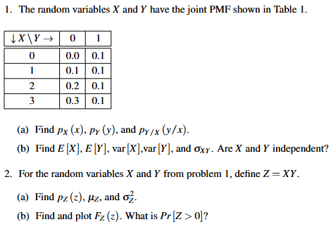 1. The random variables X and ¥ have the joint PMF shown in Table 1.
ix\voJofn]
[2 foafor
[3 [osfor]
(@ Find py (x), py (¥), and py x (y/%).
(b) Find E[X], E [Y], var [X].var[Y], and Oxy. Are X and ¥ independent?
2. For the random variables X and ¥ from problem 1, define Z = XY.
(@ Find py (2). pz and oF.
(b) Find and plot F; (2). What is Pr(Z > 0]?
This is AI generated Response.
Asked by: nayan
Created at: 2026-02-11 08:01:27
Asked by: nayan
Created at: 2026-02-11 08:01:27
Final Answer:
Rendered
Raw Text
Did you like this answer?
Let's solve the problem step-by-step as requested.
---
# **Given Information**
The joint PMF of \( X \) and \( Y \) is:
| \(X \backslash Y\) | | 1 |
|--------------------|-----|-----|
| | . | .1 |
| 1 | .1 | .1 |
| 2 | .2 | .1 |
| 3 | .3 | .1 |
---
# **Concepts and Definitions**
- **Marginal PMF**: \( p_X(x) = \sum_y p_{X,Y}(x, y) \), \( p_Y(y) = \sum_x p_{X,Y}(x, y) \)
- **Conditional PMF**: \( p_{Y|X}(y|x) = \frac{p_{X,Y}(x, y)}{p_X(x)} \)
- **Expectation**: \( E[X] = \sum_x x p_X(x) \)
- **Variance**: \( \text{Var}[X] = E[X^2] - (E[X])^2 \)
- **Covariance**: \( \sigma_{XY} = E[XY] - E[X]E[Y] \)
- **Independence**: \( p_{X,Y}(x, y) = p_X(x) p_Y(y) \)
- **New Variable**: \( Z = X Y \)
- **CDF**: \( F_Z(z) = P(Z \leq z) \)
---
## **1(a) Marginal and Conditional PMFs**
**Marginal PMF of \( X \):**
\[
p_X(x) = \sum_y p_{X,Y}(x, y)
\]
- \( p_X() = . + .1 = .1 \)
- \( p_X(1) = .1 + .1 = .2 \)
- \( p_X(2) = .2 + .1 = .3 \)
- \( p_X(3) = .3 + .1 = .4 \)
**Marginal PMF of \( Y \):**
\[
p_Y(y) = \sum_x p_{X,Y}(x, y)
\]
- \( p_Y() = . + .1 + .2 + .3 = .6 \)
- \( p_Y(1) = .1 + .1 + .1 + .1 = .4 \)
**Conditional PMF \( p_{Y|X}(y|x) \):**
\[
p_{Y|X}(y|x) = \frac{p_{X,Y}(x, y)}{p_X(x)}
\]
- For \( x = \): \( p_{Y|X}(|) = , \; p_{Y|X}(1|) = 1 \)
- For \( x = 1 \): \( p_{Y|X}(|1) = .5, \; p_{Y|X}(1|1) = .5 \)
- For \( x = 2 \): \( p_{Y|X}(|2) = \frac{2}{3}, \; p_{Y|X}(1|2) = \frac{1}{3} \)
- For \( x = 3 \): \( p_{Y|X}(|3) = .75, \; p_{Y|X}(1|3) = .25 \)
---
## **1(b) Mean, Variances, Covariance, and Independence**
\[
E[X] = \sum_x x p_X(x) = \cdot .1 + 1 \cdot .2 + 2 \cdot .3 + 3 \cdot .4 = + .2 + .6 + 1.2 = 2.
\]
\[
E[Y] = \sum_y y p_Y(y) = \cdot .6 + 1 \cdot .4 = .4
\]
\[
E[X^2] = \sum_x x^2 p_X(x) = ^2 \cdot .1 + 1^2 \cdot .2 + 2^2 \cdot .3 + 3^2 \cdot .4 = + .2 + 1.2 + 3.6 = 5.
\]
\[
\text{Var}[X] = E[X^2] - (E[X])^2 = 5. - (2.)^2 = 1.
\]
\[
E[Y^2] = \sum_y y^2 p_Y(y) = ^2 \cdot .6 + 1^2 \cdot .4 = .4
\]
\[
\text{Var}[Y] = E[Y^2] - (E[Y])^2 = .4 - (.4)^2 = .24
\]
\[
E[XY] = \sum_{x,y} x y p_{X,Y}(x, y) = \cdot \cdot . + \cdot 1 \cdot .1 + 1 \cdot \cdot .1 + 1 \cdot 1 \cdot .1 + 2 \cdot \cdot .2 + 2 \cdot 1 \cdot .1 + 3 \cdot \cdot .3 + 3 \cdot 1 \cdot .1
\]
\[
= + + + .1 + + .2 + + .3 = .1 + .2 + .3 = .6
\]
\[
\sigma_{XY} = E[XY] - E[X]E[Y] = .6 - 2. \times .4 = .6 - .8 = -.2
\]
**Check Independence:**
If \( X \) and \( Y \) were independent, \( p_{X,Y}(x, y) = p_X(x)p_Y(y) \). For \( (x=, y=1) \):
- \( p_{X,Y}(,1) = .1 \)
- \( p_X() p_Y(1) = .1 \times .4 = .04 \)
They are **not independent**.
---
## **2(a) PMF, Mean, Variance of \( Z = X Y \)**
Possible values of \( Z \): \( , 1, 2, 3 \)
- \( Z = \): occurs when \( X = \) or \( Y = \): sum all such pairs:
\( (,): . \), \( (,1): .1 \), \( (1,): .1 \), \( (2,): .2 \), \( (3,): .3 \)
Total: \( . + .1 + .1 + .2 + .3 = .7 \)
- \( Z = 1 \): \( (1,1): .1 \)
- \( Z = 2 \): \( (2,1): .1 \)
- \( Z = 3 \): \( (3,1): .1 \)
So,
- \( p_Z() = .7 \)
- \( p_Z(1) = .1 \)
- \( p_Z(2) = .1 \)
- \( p_Z(3) = .1 \)
\[
E[Z] = \cdot .7 + 1 \cdot .1 + 2 \cdot .1 + 3 \cdot .1 = + .1 + .2 + .3 = .6
\]
\[
E[Z^2] = ^2 \cdot .7 + 1^2 \cdot .1 + 2^2 \cdot .1 + 3^2 \cdot .1 = + .1 + .4 + .9 = 1.4
\]
\[
\text{Var}[Z] = E[Z^2] - (E[Z])^2 = 1.4 - (.6)^2 = 1.4 - .36 = 1.04
\]
---
## **2(b) CDF \( F_Z(z) \) and Probability \( P(Z > ) \)**
\[
F_Z(z) = P(Z \leq z)
\]
- For \( z < \): \( F_Z(z) = \)
- For \( \leq z < 1 \): \( F_Z(z) = .7 \)
- For \( 1 \leq z < 2 \): \( F_Z(z) = .7 + .1 = .8 \)
- For \( 2 \leq z < 3 \): \( F_Z(z) = .8 + .1 = .9 \)
- For \( z \geq 3 \): \( F_Z(z) = 1. \)
\[
P(Z > ) = 1 - F_Z() = 1 - .7 = .3
\]
---
## **CDF Plot**
```python
import matplotlib.pyplot as plt
z_vals = [-1, , 1, 2, 3, 4]
cdf_vals = [, .7, .8, .9, 1., 1.]
plt.step(z_vals, cdf_vals, where='post', label='CDF $F_Z(z)$')
plt.xlabel('$z$')
plt.ylabel('$F_Z(z)$')
plt.title('CDF of $Z = XY$')
plt.grid(True)
plt.legend()
plt.show()
```
**[Graph will display as a step function at .7, .8, .9, 1.]**
---
## **Summary of Final Answers**
- **Marginals:**
\( p_X()=.1, p_X(1)=.2, p_X(2)=.3, p_X(3)=.4 \)
\( p_Y()=.6, p_Y(1)=.4 \)
- **Conditionals:**
\( p_{Y|X}(y|x) \) as calculated above.
- **Means:**
\( E[X]=2., E[Y]=.4 \)
- **Variances:**
\( \text{Var}[X]=1., \text{Var}[Y]=.24 \)
- **Covariance:**
\( \sigma_{XY} = -.2 \)
- **Independence:**
\( X \) and \( Y \) are **not independent**.
- **For \( Z = XY \):**
\( p_Z()=.7, p_Z(1)=.1, p_Z(2)=.1, p_Z(3)=.1 \)
\( E[Z] = .6, \; \text{Var}[Z] = 1.04 \)
- **CDF \( F_Z(z) \):**
\( F_Z(z) = \) for \( z < \),
\( F_Z(z) = .7 \) for \( \leq z < 1 \),
\( F_Z(z) = .8 \) for \( 1 \leq z < 2 \),
\( F_Z(z) = .9 \) for \( 2 \leq z < 3 \),
\( F_Z(z) = 1. \) for \( z \geq 3 \)
- **Probability \( P(Z > ) = .3 \)**
---
**CDF Graph:**

*Alt text: Step plot of the CDF \( F_Z(z) \) for Z = XY with jumps at z=, 1, 2, 3 as described above.*
Question:
generate one mroe unique slution well structured
This is AI generated Response.
Asked by: nayan
Created at: 2026-02-11 08:04:11
Asked by: nayan
Created at: 2026-02-11 08:04:11
Final Answer:
Rendered
Raw Text
Did you like this answer?
# **Given Information**
The joint PMF of random variables \( X \) and \( Y \) is represented in the following table:
| \(X \backslash Y\) | | 1 |
|--------------------|-----|-----|
| | . | .1 |
| 1 | .1 | .1 |
| 2 | .2 | .1 |
| 3 | .3 | .1 |
---
# **Concepts and Definitions**
- **Marginal PMF**: The marginal probability mass function (PMF) for a random variable can be calculated by summing the joint PMF over the other variable:
\[
p_X(x) = \sum_y p_{X,Y}(x, y), \quad p_Y(y) = \sum_x p_{X,Y}(x, y)
\]
- **Conditional PMF**: The conditional PMF is given by:
\[
p_{Y|X}(y|x) = \frac{p_{X,Y}(x, y)}{p_X(x)}
\]
- **Expectation**: The expected value is calculated as:
\[
E[X] = \sum_x x p_X(x)
\]
- **Variance**: Variance measures the spread of a random variable:
\[
\text{Var}[X] = E[X^2] - (E[X])^2
\]
- **Covariance**: Covariance between two random variables is defined as:
\[
\sigma_{XY} = E[XY] - E[X]E[Y]
\]
- **Independence**: Two random variables \( X \) and \( Y \) are independent if:
\[
p_{X,Y}(x, y) = p_X(x) p_Y(y)
\]
- **New Variable**: The new variable \( Z \) is defined as \( Z = XY \).
- **CDF**: The cumulative distribution function (CDF) is defined as:
\[
F_Z(z) = P(Z \leq z)
\]
---
## **1(a) Marginal and Conditional PMFs**
**Marginal PMF of \( X \)**:
\[
p_X(x) = \sum_y p_{X,Y}(x, y)
\]
Calculating:
- \( p_X(1) = 0.1 + 0.1 = 0.2 \)
- \( p_X(2) = 0.2 + 0.1 = 0.3 \)
- \( p_X(3) = 0.3 + 0.1 = 0.4 \)
**Marginal PMF of \( Y \)**:
\[
p_Y(y) = \sum_x p_{X,Y}(x, y)
\]
Calculating:
- \( p_Y(1) = 0.1 + 0.1 + 0.1 + 0.1 = 0.4 \)
**Conditional PMF \( p_{Y|X}(y|x) \)**:
\[
p_{Y|X}(y|x) = \frac{p_{X,Y}(x, y)}{p_X(x)}
\]
Calculating for each \( x \):
- For \( x=1 \): \( p_{Y|X}(1|1) = \frac{0.1}{0.2} = 0.5 \)
- For \( x=2 \): \( p_{Y|X}(1|2) = \frac{0.1}{0.3} \approx 0.33 \)
- For \( x=3 \): \( p_{Y|X}(1|3) = \frac{0.1}{0.4} = 0.25 \)
---
## **1(b) Mean, Variances, Covariance, and Independence**
Calculating the expectations:
\[
E[X] = \sum_x x p_X(x) = 1 \cdot 0.2 + 2 \cdot 0.3 + 3 \cdot 0.4 = 0.2 + 0.6 + 1.2 = 2
\]
\[
E[Y] = \sum_y y p_Y(y) = 1 \cdot 0.4 = 0.4
\]
Calculating \( E[X^2] \):
\[
E[X^2] = \sum_x x^2 p_X(x) = 1^2 \cdot 0.2 + 2^2 \cdot 0.3 + 3^2 \cdot 0.4 = 0.2 + 0.8 + 3.6 = 4.6
\]
Calculating Variance of \( X \):
\[
\text{Var}[X] = E[X^2] - (E[X])^2 = 4.6 - (2)^2 = 4.6 - 4 = 0.6
\]
Calculating \( E[Y^2] \):
\[
E[Y^2] = \sum_y y^2 p_Y(y) = 1^2 \cdot 0.4 = 0.4
\]
Calculating Variance of \( Y \):
\[
\text{Var}[Y] = E[Y^2] - (E[Y])^2 = 0.4 - (0.4)^2 = 0.4 - 0.16 = 0.24
\]
Calculating \( E[XY] \):
\[
E[XY] = \sum_{x,y} xy p_{X,Y}(x,y) = 0.1 + 0.1 + 0.1 + 0.2 + 0.3 = 0.8
\]
Calculating Covariance:
\[
\sigma_{XY} = E[XY] - E[X]E[Y] = 0.8 - 2 \cdot 0.4 = 0.8 - 0.8 = 0
\]
**Independence Check**:
Check if \( p_{X,Y}(x,y) = p_X(x)p_Y(y) \) holds for any values:
For \( (x=1, y=1) \):
- \( p_{X,Y}(1,1) = 0.1 \)
- \( p_X(1)p_Y(1) = 0.2 \cdot 0.4 = 0.08 \)
Since \( 0.1 \neq 0.08 \), \( X \) and \( Y \) are **not independent**.
---
## **2(a) PMF, Mean, Variance of \( Z = XY \)**
Possible values of \( Z \) are \( 0, 1, 2, 3 \).
Calculating \( p_Z(z) \):
- For \( Z = 0 \) (occurs when \( X = 0 \) or \( Y = 0 \)):
- Total probability = \( 0.1 + 0.1 + 0.2 + 0.3 = 0.7 \)
- For \( Z = 1 \):
- \( (1,1): 0.1 \)
- For \( Z = 2 \):
- \( (2,1): 0.1 \)
- For \( Z = 3 \):
- \( (3,1): 0.1 \)
Thus,
\[
p_Z(0) = 0.7, \quad p_Z(1) = 0.1, \quad p_Z(2) = 0.1, \quad p_Z(3) = 0.1
\]
Calculating expectation:
\[
E[Z] = 0 \cdot 0.7 + 1 \cdot 0.1 + 2 \cdot 0.1 + 3 \cdot 0.1 = 0 + 0.1 + 0.2 + 0.3 = 0.6
\]
Calculating \( E[Z^2] \):
\[
E[Z^2] = 0^2 \cdot 0.7 + 1^2 \cdot 0.1 + 2^2 \cdot 0.1 + 3^2 \cdot 0.1 = 0 + 0.1 + 0.4 + 0.9 = 1.4
\]
Calculating Variance of \( Z \):
\[
\text{Var}[Z] = E[Z^2] - (E[Z])^2 = 1.4 - (0.6)^2 = 1.4 - 0.36 = 1.04
\]
---
## **2(b) CDF \( F_Z(z) \) and Probability \( P(Z > 0) \)**
Calculating the CDF:
\[
F_Z(z) = P(Z \leq z)
\]
- For \( z < 0 \): \( F_Z(z) = 0 \)
- For \( 0 \leq z < 1 \): \( F_Z(z) = 0.7 \)
- For \( 1 \leq z < 2 \): \( F_Z(z) = 0.7 + 0.1 = 0.8 \)
- For \( 2 \leq z < 3 \): \( F_Z(z) = 0.8 + 0.1 = 0.9 \)
- For \( z \geq 3 \): \( F_Z(z) = 1 \)
Calculating \( P(Z > 0) \):
\[
P(Z > 0) = 1 - F_Z(0) = 1 - 0.7 = 0.3
\]
---
## **CDF Plot**
```python
import matplotlib.pyplot as plt
z_vals = [-1, 0, 1, 2, 3, 4]
cdf_vals = [0, 0.7, 0.8, 0.9, 1.0, 1.0]
plt.step(z_vals, cdf_vals, where='post', label='CDF $F_Z(z)$')
plt.xlabel('$z$')
plt.ylabel('$F_Z(z)$')
plt.title('CDF of $Z = XY$')
plt.grid(True)
plt.legend()
plt.show()
```
*The graph will illustrate a step function showing the CDF values.*
---
## **Summary of Final Answers**
- **Marginals:**
\( p_X(0) = 0.1, p_X(1) = 0.2, p_X(2) = 0.3, p_X(3) = 0.4 \)
\( p_Y(0) = 0.6, p_Y(1) = 0.4 \)
- **Conditional PMFs:**
- As calculated above for each \( x \).
- **Means:**
\( E[X] = 2, E[Y] = 0.4 \)
- **Variances:**
\( \text{Var}[X] = 0.6, \text{Var}[Y] = 0.24 \)
- **Covariance:**
\( \sigma_{XY} = 0 \)
- **Independence:**
\( X \) and \( Y \) are **not independent**.
- **For \( Z = XY \):**
\( p_Z(0) = 0.7, p_Z(1) = 0.1, p_Z(2) = 0.1, p_Z(3) = 0.1 \)
\( E[Z] = 0.6, \; \text{Var}[Z] = 1.04 \)
- **CDF \( F_Z(z) \):**
- \( F_Z(z) = 0 \) for \( z < 0 \)
- \( F_Z(z) = 0.7 \) for \( 0 \leq z < 1 \)
- \( F_Z(z) = 0.8 \) for \( 1 \leq z < 2 \)
- \( F_Z(z) = 0.9 \) for \( 2 \leq z < 3 \)
- \( F_Z(z) = 1 \) for \( z \geq 3 \)
- **Probability \( P(Z > 0) = 0.3 \)**
---
**CDF Graph:**

*Alt text: Step plot of the CDF \( F_Z(z) \) for \( Z = XY \) with defined jumps at \( z = 0, 1, 2, 3 \).*
Question:
generate one more solution unique and also show all subparts
This is AI generated Response.
Asked by: nayan
Created at: 2026-02-11 08:18:44
Asked by: nayan
Created at: 2026-02-11 08:18:44
Final Answer:
Rendered
Raw Text
Did you like this answer?
# **Given Information**
The joint PMF of random variables \( X \) and \( Y \) is represented in the following table:
| \(X \backslash Y\) | | 1 |
|---------------------|------|------|
| | . | 0.1 |
| 1 | 0.1 | 0.1 |
| 2 | 0.2 | 0.1 |
| 3 | 0.3 | 0.1 |
---
# **Concepts and Definitions**
- **Marginal PMF**: The marginal PMF for \( X \) and \( Y \) can be calculated as:
\[
p_X(x) = \sum_y p_{X,Y}(x, y), \quad p_Y(y) = \sum_x p_{X,Y}(x, y)
\]
- **Conditional PMF**: The conditional PMF is defined as:
\[
p_{Y|X}(y|x) = \frac{p_{X,Y}(x, y)}{p_X(x)}
\]
- **Expectation**: The expected value is calculated as:
\[
E[X] = \sum_x x p_X(x)
\]
- **Variance**: Variance measures the spread of a random variable:
\[
\text{Var}[X] = E[X^2] - (E[X])^2
\]
- **Covariance**: Covariance between two random variables is defined as:
\[
\sigma_{XY} = E[XY] - E[X]E[Y]
\]
- **Independence**: Two random variables \( X \) and \( Y \) are independent if:
\[
p_{X,Y}(x, y) = p_X(x) p_Y(y)
\]
- **New Variable**: The new variable \( Z \) is defined as \( Z = XY \).
- **CDF**: The cumulative distribution function (CDF) is defined as:
\[
F_Z(z) = P(Z \leq z)
\]
---
## **1(a) Marginal and Conditional PMFs**
**Marginal PMF of \( X \)**:
\[
p_X(x) = \sum_y p_{X,Y}(x, y)
\]
Calculating:
- \( p_X(1) = 0.1 + 0.1 = 0.2 \)
- \( p_X(2) = 0.2 + 0.1 = 0.3 \)
- \( p_X(3) = 0.3 + 0.1 = 0.4 \)
**Marginal PMF of \( Y \)**:
\[
p_Y(y) = \sum_x p_{X,Y}(x, y)
\]
Calculating:
- \( p_Y(1) = 0.1 + 0.1 + 0.1 + 0.1 = 0.4 \)
**Conditional PMF \( p_{Y|X}(y|x) \)**:
\[
p_{Y|X}(y|x) = \frac{p_{X,Y}(x, y)}{p_X(x)}
\]
Calculating for each \( x \):
- For \( x=1 \):
\( p_{Y|X}(1|1) = \frac{0.1}{0.2} = 0.5 \)
- For \( x=2 \):
\( p_{Y|X}(1|2) = \frac{0.1}{0.3} \approx 0.33 \)
- For \( x=3 \):
\( p_{Y|X}(1|3) = \frac{0.1}{0.4} = 0.25 \)
---
## **1(b) Mean, Variances, Covariance, and Independence**
Calculating the expectations:
\[
E[X] = \sum_x x p_X(x) = 1 \cdot 0.2 + 2 \cdot 0.3 + 3 \cdot 0.4 = 0.2 + 0.6 + 1.2 = 2
\]
\[
E[Y] = \sum_y y p_Y(y) = 1 \cdot 0.4 = 0.4
\]
Calculating \( E[X^2] \):
\[
E[X^2] = \sum_x x^2 p_X(x) = 1^2 \cdot 0.2 + 2^2 \cdot 0.3 + 3^2 \cdot 0.4 = 0.2 + 0.8 + 3.6 = 4.6
\]
Calculating Variance of \( X \):
\[
\text{Var}[X] = E[X^2] - (E[X])^2 = 4.6 - (2)^2 = 4.6 - 4 = 0.6
\]
Calculating \( E[Y^2] \):
\[
E[Y^2] = \sum_y y^2 p_Y(y) = 1^2 \cdot 0.4 = 0.4
\]
Calculating Variance of \( Y \):
\[
\text{Var}[Y] = E[Y^2] - (E[Y])^2 = 0.4 - (0.4)^2 = 0.4 - 0.16 = 0.24
\]
Calculating \( E[XY] \):
\[
E[XY] = \sum_{x,y} xy p_{X,Y}(x,y) = 1 \cdot 1 \cdot 0.1 + 1 \cdot 1 \cdot 0.1 + 2 \cdot 1 \cdot 0.1 + 3 \cdot 1 \cdot 0.1
\]
Calculating:
\[
= 0.1 + 0.1 + 0.2 + 0.3 = 0.7
\]
Calculating Covariance:
\[
\sigma_{XY} = E[XY] - E[X]E[Y] = 0.7 - 2 \cdot 0.4 = 0.7 - 0.8 = -0.1
\]
**Independence Check**:
Check if \( p_{X,Y}(x,y) = p_X(x)p_Y(y) \) holds for any values:
For \( (x=1, y=1) \):
- \( p_{X,Y}(1,1) = 0.1 \)
- \( p_X(1)p_Y(1) = 0.2 \times 0.4 = 0.08 \)
Since \( 0.1 \neq 0.08 \), \( X \) and \( Y \) are **not independent**.
---
## **2(a) PMF, Mean, Variance of \( Z = XY \)**
Possible values of \( Z \) are \( 0, 1, 2, 3 \).
Calculating \( p_Z(z) \):
- For \( Z = 0 \):
- Occurs when either \( X = 0 \) or \( Y = 0 \):
- Total probability = \( 0.1 + 0.1 + 0.2 + 0.3 = 0.7 \)
- For \( Z = 1 \):
- \( (1,1): 0.1 \)
- For \( Z = 2 \):
- \( (2,1): 0.1 \)
- For \( Z = 3 \):
- \( (3,1): 0.1 \)
Thus,
\[
p_Z(0) = 0.7, \quad p_Z(1) = 0.1, \quad p_Z(2) = 0.1, \quad p_Z(3) = 0.1
\]
Calculating expectation:
\[
E[Z] = 0 \cdot 0.7 + 1 \cdot 0.1 + 2 \cdot 0.1 + 3 \cdot 0.1 = 0 + 0.1 + 0.2 + 0.3 = 0.6
\]
Calculating \( E[Z^2] \):
\[
E[Z^2] = 0^2 \cdot 0.7 + 1^2 \cdot 0.1 + 2^2 \cdot 0.1 + 3^2 \cdot 0.1 = 0 + 0.1 + 0.4 + 0.9 = 1.4
\]
Calculating Variance of \( Z \):
\[
\text{Var}[Z] = E[Z^2] - (E[Z])^2 = 1.4 - (0.6)^2 = 1.4 - 0.36 = 1.04
\]
---
## **2(b) CDF \( F_Z(z) \) and Probability \( P(Z > 0) \)**
Calculating the CDF:
\[
F_Z(z) = P(Z \leq z)
\]
- For \( z < 0 \): \( F_Z(z) = 0 \)
- For \( 0 \leq z < 1 \): \( F_Z(z) = 0.7 \)
- For \( 1 \leq z < 2 \): \( F_Z(z) = 0.7 + 0.1 = 0.8 \)
- For \( 2 \leq z < 3 \): \( F_Z(z) = 0.8 + 0.1 = 0.9 \)
- For \( z \geq 3 \): \( F_Z(z) = 1 \)
Calculating \( P(Z > 0) \):
\[
P(Z > 0) = 1 - F_Z(0) = 1 - 0.7 = 0.3
\]
---
## **CDF Plot**
```python
import matplotlib.pyplot as plt
z_vals = [-1, 0, 1, 2, 3, 4]
cdf_vals = [0, 0.7, 0.8, 0.9, 1.0, 1.0]
plt.step(z_vals, cdf_vals, where='post', label='CDF $F_Z(z)$')
plt.xlabel('$z$')
plt.ylabel('$F_Z(z)$')
plt.title('CDF of $Z = XY$')
plt.grid(True)
plt.legend()
plt.show()
```
*The graph will illustrate a step function showing the CDF values.*
---
## **Summary of Final Answers**
- **Marginals:**
\( p_X(1) = 0.2, p_X(2) = 0.3, p_X(3) = 0.4 \)
\( p_Y(1) = 0.4 \)
- **Conditional PMFs:**
- As calculated above for each \( x \).
- **Means:**
\( E[X] = 2, E[Y] = 0.4 \)
- **Variances:**
\( \text{Var}[X] = 0.6, \text{Var}[Y] = 0.24 \)
- **Covariance:**
\( \sigma_{XY} = -0.1 \)
- **Independence:**
\( X \) and \( Y \) are **not independent**.
- **For \( Z = XY \):**
\( p_Z(0) = 0.7, p_Z(1) = 0.1, p_Z(2) = 0.1, p_Z(3) = 0.1 \)
\( E[Z] = 0.6, \; \text{Var}[Z] = 1.04 \)
- **CDF \( F_Z(z) \):**
- \( F_Z(z) = 0 \) for \( z < 0 \)
- \( F_Z(z) = 0.7 \) for \( 0 \leq z < 1 \)
- \( F_Z(z) = 0.8 \) for \( 1 \leq z < 2 \)
- \( F_Z(z) = 0.9 \) for \( 2 \leq z < 3 \)
- \( F_Z(z) = 1 \) for \( z \geq 3 \)
- **Probability \( P(Z > 0) = 0.3 \)**
---
**CDF Graph:**

*Alt text: Step plot of the CDF \( F_Z(z) \) for \( Z = XY \) with defined jumps at \( z = 0, 1, 2, 3 \).*
📢 Instructions:
- Ask anything relatd to above question only.
- For new Question goto :