solve coorect answerFigure P4.64 shows a fixed control volume. It has a volume V0 = 1.0 ft3, a flow area A = 1.0 ft2,
and a length £0 = 1.0 ft. Position x represents the center of the control volume where the fluid
velocity VO = 1.0 ft/s and the density p0 = 1.800 slug/ft3. Also, at position x the fluid density does
not change locally with time but decreases in the axial direction at the linear rate of 0.25 slug/ft4.
Use the system or Lagrangian approach to evaluate dp/dt. Compare this result with that of the
material derivative and flux terms.
Figure P4.64
System and control
volume at time 1
t=1
=
| ver
| —_— | A 1 [3
|=
! |
— System at time 1 + st
Question:
solve coorect answerFigure P4.64 shows a fixed control volume. It has a volume V0 = 1.0 ft3, a flow area A = 1.0 ft2,
and a length £0 = 1.0 ft. Position x represents the center of the control volume where the fluid
velocity VO = 1.0 ft/s and the density p0 = 1.800 slug/ft3. Also, at position x the fluid density does
not change locally with time but decreases in the axial direction at the linear rate of 0.25 slug/ft4.
Use the system or Lagrangian approach to evaluate dp/dt. Compare this result with that of the
material derivative and flux terms.
Figure P4.64
System and control
volume at time 1
t=1
=
| ver
| —_— | A 1 [3
|=
! |
— System at time 1 + st
This is AI generated Response.
Asked by: pooja gargunde
Created at: 2025-07-25 09:53:55
Final Answer:
RenderedRaw Text
Did you like this answer?
Let's break down and solve the problem step by step:
---
### **Given Data**
- **Control Volume (V₀):** 1.0 ft³
- **Flow Area (A):** 1.0 ft²
- **Length (ℓ₀):** 1.0 ft
- **Velocity at center (V₀):** 1.0 ft/s
- **Density at center (ρ₀):** 1.800 slug/ft³
- **Density gradient:** decreases at 0.25 slug/(ft⁴) in the axial direction (∂ρ/∂x = –0.25 slug/ft⁴)
- **No local change in density:** ∂ρ/∂t = 0
---
## **A. System (Lagrangian) Approach**
For a system, you follow the same fluid particles as they move. The rate of change of density for a particle is given by the **material derivative:**
\[
\frac{D\rho}{Dt} = \frac{\partial \rho}{\partial t} + V \frac{\partial \rho}{\partial x}
\]
Given:
- \(\frac{\partial \rho}{\partial t} = 0\)
- \(V = V_0 = 1.0\) ft/s
- \(\frac{\partial \rho}{\partial x} = -0.25\) slug/ft⁴
Plug in the values:
\[
\frac{D\rho}{Dt} = 0 + (1.0)\times (-0.25) = -0.25 \text{ slug/ft}^3\text{/s}
\]
---
## **B. Control Volume (Eulerian) Approach**
The average rate of change of density in the control volume is:
\[
\frac{d}{dt}\int_{CV} \rho \, dV = \int_{CV} \frac{\partial \rho}{\partial t} dV + \oint_{CS} \rho \vec{V} \cdot d\vec{A}
\]
But since the control volume is fixed and \(\frac{\partial \rho}{\partial t} = 0\), the time rate of change inside the CV is zero. Instead, we focus on the **flux** across the CV boundaries.
#### **Net outflow of mass (density flux):**
\[
\text{Net flux} = (\rho V A)_{out} - (\rho V A)_{in}
\]
Since area is the same on both sides, but density varies linearly in \(x\):
- At the **inlet** (left):
\(x = x_0 - \frac{\ell_0}{2}\)
- At the **outlet** (right):
\(x = x_0 + \frac{\ell_0}{2}\)
So,
\[
\rho_{in} = \rho_0 + \frac{\partial \rho}{\partial x} \left(-\frac{\ell_0}{2}\right)
= 1.800 + (-0.25) \times \left(-\frac{1}{2}\right)
= 1.800 + 0.125 = 1.925 \text{ slug/ft}^3
\]
\[
\rho_{out} = \rho_0 + \frac{\partial \rho}{\partial x} \left(\frac{\ell_0}{2}\right)
= 1.800 + (-0.25) \times \left(\frac{1}{2}\right)
= 1.800 - 0.125 = 1.675 \text{ slug/ft}^3
\]
Assume the velocity is constant (V₀):
\[
\text{Net mass flux} = (\rho_{out} V_0 A) - (\rho_{in} V_0 A)
\]
\[
= [1.675 \times 1.0 \times 1.0] - [1.925 \times 1.0 \times 1.0]
= 1.675 - 1.925 = -0.25 \text{ slug/s}
\]
Divide by the control volume \(V_0\) to get the rate of change of average density:
\[
\frac{d\overline{\rho}}{dt} = \frac{\text{Net mass flux}}{V_0}
= \frac{-0.25}{1.0}
= -0.25 \text{ slug/ft}^3\text{/s}
\]
---
## **C. Comparison**
Both the **system (material derivative)** and the **control volume (flux)** approaches yield:
\[
\boxed{
\frac{d\rho}{dt} = -0.25 \text{ slug/ft}^3\text{/s}
}
\]
This shows consistency between the Lagrangian (system) and Eulerian (control volume) analyses.
---
### **Summary Table**
| Approach | Result for \( \frac{d\rho}{dt} \) |
|---------------|:---------------------------------:|
| System/Lagrangian | \(-0.25 \text{ slug/ft}^3\text{/s}\) |
| Control Volume | \(-0.25 \text{ slug/ft}^3\text{/s}\) |
If you need a step-by-step derivation or further explanation of any step, let me know!
Question:
Consider the equation below. f
(
x
)
=
4
x
3
+
2
1
x
2
−
2
9
4
x
+
2
(
a
)
Find the intervals on which f is increasing.
(
Enter your answer using interval notation.
)
Find the interval on which f is decreasing.
(
Enter your answer using interval notation.
)
(
b
)
Find the local minimum and maximum values of f
.
local minimum value local maximum value
(
c
)
Find the inflection point.
(
x
,
y
)
=
Find the interval on which f is concave up
.
(
Enter your answer using interval notation.
)
Find the interval on which f is concave down.
(
Enter your answer using interval notation.
) solve correct answer
This is AI generated Response.
Asked by: pooja gargunde
Created at: 2025-07-25 11:49:17
VIPSolutions focuses on clear, step‑by‑step explanations so you can learn quickly. Whether you need an AI‑generated walkthrough or a short hint to get unstuck, each solution is organized for fast reading and easy review later.
Search similar questions, compare approaches, and bookmark the best answers for revision. Our goal is simple: quick, reliable study help that feels natural—not noisy.
 VIPSolutions
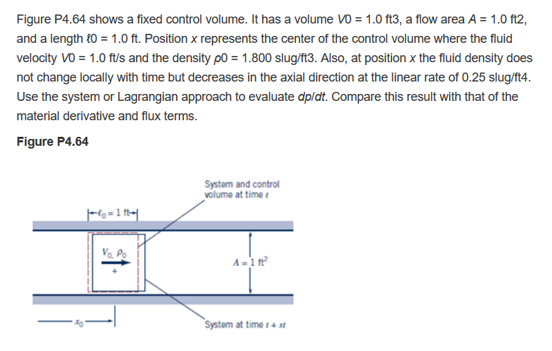 Figure P4.64 shows a fixed control volume. It has a volume V0 = 1.0 ft3, a flow area A = 1.0 ft2,
and a length £0 = 1.0 ft. Position x represents the center of the control volume where the fluid
velocity VO = 1.0 ft/s and the density p0 = 1.800 slug/ft3. Also, at position x the fluid density does
not change locally with time but decreases in the axial direction at the linear rate of 0.25 slug/ft4.
Use the system or Lagrangian approach to evaluate dp/dt. Compare this result with that of the
material derivative and flux terms.
Figure P4.64
System and control
volume at time 1
t=1
=
| ver
| —_— | A 1 [3
|=
! |
— System at time 1 + st