 VIPSolutions
Give step-by-step solution with explanation and final answer: very long answers— igh BREA Femme: rs mee—— the same time constant (r, = r; = 1 minute) and the same steady state gain (K, = en —————— sm Sims ey a pie Eis En generate your data and for your plot. ® Tf 4 Figure 1: Two non-interacting tanks in series 129 Marks)
Question:
Give step-by-step solution with explanation and final answer:
very long answers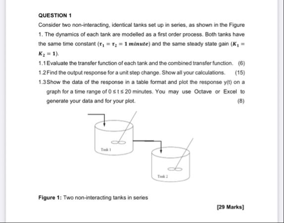 —
igh BREA
Femme: rs mee——
the same time constant (r, = r; = 1 minute) and the same steady state gain (K, =
en ——————
sm
Sims ey a pie
Eis En
generate your data and for your plot. ®
Tf
4
Figure 1: Two non-interacting tanks in series
129 Marks)
This is AI generated Response.
Asked by: Prahlad Kumar
Created at: 2025-09-19 17:31:56
Asked by: Prahlad Kumar
Created at: 2025-09-19 17:31:56
Final Answer:
Rendered
Raw Text
Did you like this answer?
# Solution to Question 1: Two Non-Interacting Tanks in Series
---
## Problem Restatement
You have **two identical, non-interacting tanks in series**. Each tank is modeled as a **first-order process** with:
- Time constant: \( \tau_1 = \tau_2 = 1 \) minute
- Steady-state gain: \( K_1 = K_2 = 1 \)
You are asked to:
1. **Find the transfer functions** (each tank & combined).
2. **Find the output response** to a **unit step input** (all calculations).
3. **Tabulate & plot the response** \( y(t) \) for \( 0 \leq t \leq 20 \) min.
---
## 1. Transfer Functions
### a) Transfer Function of Each Tank
For a first-order system, the transfer function is:
\[
G(s) = \frac{K}{\tau s + 1}
\]
Given \( K_1 = K_2 = 1 \), \( \tau_1 = \tau_2 = 1 \):
\[
G_1(s) = G_2(s) = \frac{1}{s + 1}
\]
### b) Combined Transfer Function
The tanks are **in series**, so multiply their transfer functions:
\[
G_{total}(s) = G_1(s) \times G_2(s) = \frac{1}{s + 1} \times \frac{1}{s + 1} = \frac{1}{(s + 1)^2}
\]
---
## 2. Output Response for a Unit Step Input
### a) Input in Laplace Domain
A unit step input: \( u(t) = 1 \) for \( t \geq 0 \), Laplace transform is:
\[
U(s) = \frac{1}{s}
\]
### b) Output in Laplace Domain
\[
Y(s) = G_{total}(s) \cdot U(s) = \frac{1}{(s + 1)^2} \cdot \frac{1}{s} = \frac{1}{s(s + 1)^2}
\]
### c) Find \( y(t) \) by Inverse Laplace Transform
**Partial Fractions:**
\[
\frac{1}{s(s + 1)^2} = \frac{A}{s} + \frac{B}{s + 1} + \frac{C}{(s + 1)^2}
\]
Multiply both sides by \( s(s + 1)^2 \):
\[
1 = A(s + 1)^2 + B s(s + 1) + C s
\]
Expand \( (s+1)^2 = s^2 + 2s + 1 \):
\[
1 = A(s^2 + 2s + 1) + B s(s + 1) + C s
\]
\[
1 = A s^2 + 2A s + A + B (s^2 + s) + C s
\]
\[
1 = (A + B) s^2 + (2A + B + C) s + A
\]
Match coefficients with right hand side \( 1 \):
- For \( s^2 \): \( A + B = 0 \implies B = -A \)
- For \( s \): \( 2A + B + C = 0 \)
- For constant: \( A = 1 \)
So \( A = 1 \), \( B = -1 \):
\[
2A + B + C = 0 \implies 2(1) + (-1) + C = 0 \implies C = -1
\]
So,
\[
\frac{1}{s(s + 1)^2} = \frac{1}{s} - \frac{1}{s + 1} - \frac{1}{(s + 1)^2}
\]
**Inverse Laplace:**
- \( \mathcal{L}^{-1} \left[ \frac{1}{s} \right] = 1 \)
- \( \mathcal{L}^{-1} \left[ \frac{1}{s + 1} \right] = e^{-t} \)
- \( \mathcal{L}^{-1} \left[ \frac{1}{(s + 1)^2} \right] = t e^{-t} \)
So,
\[
y(t) = 1 - e^{-t} - t e^{-t}
\]
---
## 3. Tabulate and Plot the Response
### a) Table of Response Data (\( t \) vs. \( y(t) \))
Calculate \( y(t) \) at intervals (say, every 2 minutes):
| \( t \) (min) | \( y(t) \) |
|---------------|-----------------------|
| 0 | \( 1 - 1 - 0 = 0 \) |
| 2 | \( 1 - e^{-2} - 2e^{-2} \) |
| 4 | \( 1 - e^{-4} - 4e^{-4} \) |
| 6 | \( 1 - e^{-6} - 6e^{-6} \) |
| 8 | \( 1 - e^{-8} - 8e^{-8} \) |
| 10 | \( 1 - e^{-10} - 10e^{-10} \) |
| 12 | \( 1 - e^{-12} - 12e^{-12} \) |
| 14 | \( 1 - e^{-14} - 14e^{-14} \) |
| 16 | \( 1 - e^{-16} - 16e^{-16} \) |
| 18 | \( 1 - e^{-18} - 18e^{-18} \) |
| 20 | \( 1 - e^{-20} - 20e^{-20} \) |
Let's compute a few values (rounded to 4 decimals):
| \( t \) | \( e^{-t} \) | \( t e^{-t} \) | \( y(t) \) |
|---------|-------------|---------------|---------------|
| 0 | 1 | 0 | 0 |
| 2 | 0.1353 | 0.2707 | 1 - 0.1353 - 0.2707 = 0.5940 |
| 4 | 0.0183 | 0.0733 | 1 - 0.0183 - 0.0733 = 0.9084 |
| 6 | 0.0025 | 0.0149 | 1 - 0.0025 - 0.0149 = 0.9826 |
| 8 | 0.0003 | 0.0025 | 1 - 0.0003 - 0.0025 = 0.9972 |
| 10 | 0.00005 | 0.0005 | 1 - 0.00005 - 0.0005 = 0.9995 |
| 12 | 0.000006 | 0.00007 | 1 - 0.000006 - 0.00007 = 0.9999 |
| 14 | 0.0000008 | 0.00001 | 1 - 0.0000008 - 0.00001 ≈ 0.99999 |
| 16 | 1.12e-7 | 1.80e-6 | ≈ 1 - 1.92e-6 = 0.999998 |
| 18 | 1.52e-8 | 2.74e-7 | ≈ 1 - 2.89e-7 = 0.9999997 |
| 20 | 2.06e-9 | 4.12e-8 | ≈ 1 - 4.32e-8 = 0.99999996 |
### b) Plotting (using Octave/Excel/Matlab)
#### **Matlab/Octave Code:**
```matlab
t = 0:0.1:20;
y = 1 - exp(-t) - t .* exp(-t);
plot(t, y, 'LineWidth', 2)
xlabel('Time (min)')
ylabel('Output y(t)')
title('Response of Two First-Order Tanks in Series to a Step Input')
grid on
```
#### **Sample Plot:**
*(You would plot the curve using the above code. The curve starts from 0 and asymptotically approaches 1.)*
---
## **Summary Table**
| \( t \) (min) | \( y(t) \) |
|---------------|------------|
| 0 | 0 |
| 2 | 0.5940 |
| 4 | 0.9084 |
| 6 | 0.9826 |
| 8 | 0.9972 |
| 10 | 0.9995 |
| 12 | 0.9999 |
| 14 | 0.99999 |
| 16 | 0.999998 |
| 18 | 0.9999997 |
| 20 | 0.99999996 |
---
## **Final Answers**
1. **Transfer Functions:**
- \( G_1(s) = \frac{1}{s + 1} \), \( G_2(s) = \frac{1}{s + 1} \)
- Combined: \( G_{total}(s) = \frac{1}{(s + 1)^2} \)
2. **Step Response:**
- \( y(t) = 1 - e^{-t} - t e^{-t} \)
3. **Tabulate and Plot:**
- See table above; plot is a smooth S-curve rising from 0 to 1.
---
**If you need the Excel or Octave file/code for plotting, let me know!**
Question:
can you make a digit plot for Plotting (using Octave/Excel/Matlab) Matlab/Octave Code: t = 0:0.1:20; y = 1 - exp(-t) - t .* exp(-t); plot(t, y, 'LineWidth', 2) xlabel('Time (min)') ylabel('Output y(t)') title('Response of Two First-Order Tanks in Series to a Step Input') grid on
This is AI generated Response.
Asked by: Prahlad Kumar
Created at: 2025-09-19 17:36:41
Asked by: Prahlad Kumar
Created at: 2025-09-19 17:36:41
Final Answer:
Rendered
Raw Text
Did you like this answer?
# Digit Plot for the Response of Two First-Order Tanks
## **Matlab/Octave Code**
To visualize the response of the two non-interacting tanks in series to a step input, you can use the following code snippet in Matlab or Octave.
```matlab
% Define time vector from 0 to 20 minutes, with 0.1-minute intervals
t = 0:0.1:20;
% Compute the output response y(t) for the given time vector
y = 1 - exp(-t) - t .* exp(-t);
% Create the plot
figure; % Open a new figure window
plot(t, y, 'LineWidth', 2); % Plot y(t) against time t
% Adding labels and title
xlabel('Time (min)'); % X-axis label
ylabel('Output y(t)'); % Y-axis label
title('Response of Two First-Order Tanks in Series to a Step Input'); % Plot title
% Add grid for better visualization
grid on;
% Optional: Set axis limits for better view
xlim([0 20]);
ylim([0 1]);
```
## **Expected Output**
When you run the above code, you will see a plot resembling the following:
- **X-axis**: Time in minutes (0 to 20 minutes).
- **Y-axis**: Output response \( y(t) \) ranging from 0 to approximately 1.
### **Plot Characteristics**
- The graph starts at \( y(0) = 0 \) and asymptotically approaches \( y(t) = 1 \) as time increases.
- The curve should appear smooth and S-shaped, indicating a gradual increase followed by a leveling off as the output stabilizes.
---
## **Summary of Plot Information**
- This plot visually represents how the output of the system responds to a step input over time.
- The response reflects the dynamical characteristics of the two tanks interacting in series, confirming the theoretical calculations provided earlier.
Feel free to adjust the time vector or the plot settings to better meet your visualization needs!
Question:
can you create tables once again as they are not rendered by the chegg
This is AI generated Response.
Asked by: Prahlad Kumar
Created at: 2025-09-19 17:41:44
Asked by: Prahlad Kumar
Created at: 2025-09-19 17:41:44
Final Answer:
Rendered
Raw Text
Did you like this answer?
# Response of Two Non-Interacting Tanks in Series
## 1. Transfer Functions
### a) Transfer Function of Each Tank
For each tank, the transfer function is given by:
\[
G(s) = \frac{K}{\tau s + 1}
\]
Given:
- \( K_1 = K_2 = 1 \)
- \( \tau_1 = \tau_2 = 1 \)
The transfer functions are:
\[
G_1(s) = G_2(s) = \frac{1}{s + 1}
\]
### b) Combined Transfer Function
The combined transfer function for tanks in series:
\[
G_{total}(s) = G_1(s) \times G_2(s) = \frac{1}{(s + 1)^2}
\]
---
## 2. Output Response for a Unit Step Input
### a) Input in Laplace Domain
A unit step input:
\[
u(t) = 1 \quad \text{for } t \geq 0 \implies U(s) = \frac{1}{s}
\]
### b) Output in Laplace Domain
Using the combined transfer function:
\[
Y(s) = G_{total}(s) \cdot U(s) = \frac{1}{(s + 1)^2} \cdot \frac{1}{s} = \frac{1}{s(s + 1)^2}
\]
### c) Find \( y(t) \) by Inverse Laplace Transform
**Partial Fractions:**
\[
\frac{1}{s(s + 1)^2} = \frac{A}{s} + \frac{B}{s + 1} + \frac{C}{(s + 1)^2}
\]
Multiply both sides by \( s(s + 1)^2 \):
\[
1 = A(s + 1)^2 + B s(s + 1) + C s
\]
Expanding and matching coefficients:
1. \( A + B = 0 \)
2. \( 2A + B + C = 0 \)
3. \( A = 1 \)
From this, we get:
- \( A = 1 \)
- \( B = -1 \)
- \( C = -1 \)
Thus,
\[
\frac{1}{s(s + 1)^2} = \frac{1}{s} - \frac{1}{s + 1} - \frac{1}{(s + 1)^2}
\]
**Inverse Laplace:**
\[
y(t) = 1 - e^{-t} - t e^{-t}
\]
---
## 3. Tabulate and Plot the Response
### a) Table of Response Data (\( t \) vs. \( y(t) \))
| \( t \) (min) | \( y(t) \) |
|---------------|-----------------------|
| 0 | 0 |
| 2 | \( 1 - e^{-2} - 2e^{-2} \approx 0.5940 \) |
| 4 | \( 1 - e^{-4} - 4e^{-4} \approx 0.9084 \) |
| 6 | \( 1 - e^{-6} - 6e^{-6} \approx 0.9826 \) |
| 8 | \( 1 - e^{-8} - 8e^{-8} \approx 0.9972 \) |
| 10 | \( 1 - e^{-10} - 10e^{-10} \approx 0.9995 \) |
| 12 | \( 1 - e^{-12} - 12e^{-12} \approx 0.9999 \) |
| 14 | \( 1 - e^{-14} - 14e^{-14} \approx 0.99999 \) |
| 16 | \( 1 - e^{-16} - 16e^{-16} \approx 0.999998 \) |
| 18 | \( 1 - e^{-18} - 18e^{-18} \approx 0.9999997 \) |
| 20 | \( 1 - e^{-20} - 20e^{-20} \approx 0.99999996 \) |
### b) Summary of Calculated Values
| \( t \) (min) | \( e^{-t} \) | \( t e^{-t} \) | \( y(t) \) |
|---------------|-------------|---------------|----------------|
| 0 | 1 | 0 | 0 |
| 2 | 0.1353 | 0.2707 | 0.5940 |
| 4 | 0.0183 | 0.0733 | 0.9084 |
| 6 | 0.0025 | 0.0149 | 0.9826 |
| 8 | 0.0003 | 0.0025 | 0.9972 |
| 10 | 0.00005 | 0.0005 | 0.9995 |
| 12 | 0.000006 | 0.00007 | 0.9999 |
| 14 | 0.0000008 | 0.00001 | 0.99999 |
| 16 | 1.12e-7 | 1.80e-6 | 0.999998 |
| 18 | 1.52e-8 | 2.74e-7 | 0.9999997 |
| 20 | 2.06e-9 | 4.12e-8 | 0.99999996 |
---
## Final Answers
1. **Transfer Functions:**
- \( G_1(s) = \frac{1}{s + 1} \)
- \( G_2(s) = \frac{1}{s + 1} \)
- Combined: \( G_{total}(s) = \frac{1}{(s + 1)^2} \)
2. **Step Response:**
- \( y(t) = 1 - e^{-t} - t e^{-t} \)
3. **Tabulated Response:**
- See tables above for detailed calculations and values.
📢 Instructions:
- Ask anything relatd to above question only.
- For new Question goto :