Give step-by-step solution with each step explanation and final conclusionih RHE ii 1h Ta
Cea iil Ee
t the scanned answer copy of the following questions: ue
a i
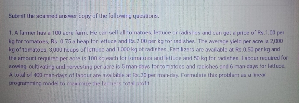
{ a Lo acre farm. He can sell all tomatoes, lettuce or radishes and can get a price of Rs.1.! 00p
natoes, fs 0.75 a heap for lettuce and Rs.2.00 per kg for radishes. The average yield per acre is 2,00
oes, 3,000 heaps of lettuce and 1,000 kg of radishes. Fertilizers are available at Rs.0.50 per g an
Ti quired per acre is 100 kg each for tomatoes and lettuce and 50 kg for radishes. Labour equi
(zthg {iidarvesting per acre is 5 man-days for tomatoes and radishes and 6 man-days fo il tt
man-da s of labour are available at Rs.20 per man-day. Formulate this problem as a linear"
n odel to m aximize the farmer's total profit Ee
hi 0 i Ht ha
Hilti Ll ASHE a
Question:
Give step-by-step solution with each step explanation and final conclusionih RHE ii 1h Ta
Cea iil Ee
t the scanned answer copy of the following questions: ue
a i
{ a Lo acre farm. He can sell all tomatoes, lettuce or radishes and can get a price of Rs.1.! 00p
natoes, fs 0.75 a heap for lettuce and Rs.2.00 per kg for radishes. The average yield per acre is 2,00
oes, 3,000 heaps of lettuce and 1,000 kg of radishes. Fertilizers are available at Rs.0.50 per g an
Ti quired per acre is 100 kg each for tomatoes and lettuce and 50 kg for radishes. Labour equi
(zthg {iidarvesting per acre is 5 man-days for tomatoes and radishes and 6 man-days fo il tt
man-da s of labour are available at Rs.20 per man-day. Formulate this problem as a linear"
n odel to m aximize the farmer's total profit Ee
hi 0 i Ht ha
Hilti Ll ASHE a
This is AI generated Response.
Asked by: Priyanshu Yadav
Created at: 2025-10-11 14:31:10
Final Answer:
RenderedRaw Text
Did you like this answer?
Let's break down and formulate the problem step-by-step:
---
# Step 1: Define Decision Variables
Let:
- \( x_1 \) = Acres allocated to **tomatoes**
- \( x_2 \) = Acres allocated to **lettuce**
- \( x_3 \) = Acres allocated to **radishes**
---
# Step 2: Objective Function (Profit Maximization)
### **Revenue:**
- Tomatoes: \( 2,000 \) kg/acre × ₹1.00/kg × \( x_1 \) acres = ₹2,000\( x_1 \)
- Lettuce: \( 3,000 \) heaps/acre × ₹.75/heap × \( x_2 \) acres = ₹2,250\( x_2 \)
- Radishes: \( 1,000 \) kg/acre × ₹2.00/kg × \( x_3 \) acres = ₹2,000\( x_3 \)
### **Fertilizer Cost:**
- Tomatoes: 100 kg/acre × ₹.50/kg × \( x_1 \) = ₹50\( x_1 \)
- Lettuce: 100 kg/acre × ₹.50/kg × \( x_2 \) = ₹50\( x_2 \)
- Radishes: 50 kg/acre × ₹.50/kg × \( x_3 \) = ₹25\( x_3 \)
### **Labour Cost:**
- Tomatoes: 5 man-days/acre × ₹20/man-day × \( x_1 \) = ₹100\( x_1 \)
- Lettuce: 6 man-days/acre × ₹20/man-day × \( x_2 \) = ₹120\( x_2 \)
- Radishes: 5 man-days/acre × ₹20/man-day × \( x_3 \) = ₹100\( x_3 \)
### **Net Profit:**
\[
\begin{align*}
\text{Tomatoes:} & \quad ₹2,000x_1 - ₹50x_1 - ₹100x_1 = ₹1,850x_1 \\
\text{Lettuce:} & \quad ₹2,250x_2 - ₹50x_2 - ₹120x_2 = ₹2,080x_2 \\
\text{Radishes:} & \quad ₹2,000x_3 - ₹25x_3 - ₹100x_3 = ₹1,875x_3 \\
\end{align*}
\]
**Total profit to maximize:**
\[
\text{Maximize:} \quad Z = 185x_1 + 208x_2 + 1875x_3
\]
---
# Step 3: Constraints
### **1. Land Constraint:**
\[
x_1 + x_2 + x_3 \leq 100
\]
### **2. Labour Constraint:**
\[
5x_1 + 6x_2 + 5x_3 \leq 400
\]
### **3. Non-negativity:**
\[
x_1 \geq ,\quad x_2 \geq ,\quad x_3 \geq
\]
---
# Step 4: Complete Linear Programming Model
\[
\begin{align*}
\text{Maximize:} \quad & Z = 185x_1 + 208x_2 + 1875x_3 \\
\text{Subject to:} \quad & x_1 + x_2 + x_3 \leq 100 \\
& 5x_1 + 6x_2 + 5x_3 \leq 400 \\
& x_1 \geq ,\ x_2 \geq ,\ x_3 \geq
\end{align*}
\]
---
# **Conclusion**
This linear programming model will help the farmer determine the optimal allocation of his 100-acre farm among tomatoes, lettuce, and radishes to **maximize the total profit**, considering land, fertilizer, and labor constraints.
If you want to solve for the actual values of \( x_1, x_2, x_3 \), you can use the simplex method or any LP solver.
Question:
add explanation after each part
This is AI generated Response.
Asked by: Priyanshu Yadav
Created at: 2025-10-11 14:32:30
Final Answer:
RenderedRaw Text
Did you like this answer?
# Step-by-Step Solution for Linear Programming Problem
## Step 1: Define Decision Variables
We begin by defining our decision variables, which represent the acres allocated to each crop:
- **\( x_1 \)**: Acres allocated to **tomatoes**
- **\( x_2 \)**: Acres allocated to **lettuce**
- **\( x_3 \)**: Acres allocated to **radishes**
This sets the foundation for the model, allowing us to quantify the areas dedicated to each crop.
---
## Step 2: Objective Function (Profit Maximization)
### Revenue Calculation
We calculate the revenue generated from each crop based on the yield per acre and the selling price:
- **Tomatoes**:
\[
\text{Revenue} = 2,000 \, \text{kg/acre} \times ₹1.00/\text{kg} \times x_1 = ₹2,000x_1
\]
- **Lettuce**:
\[
\text{Revenue} = 3,000 \, \text{heaps/acre} \times ₹0.75/\text{heap} \times x_2 = ₹2,250x_2
\]
- **Radishes**:
\[
\text{Revenue} = 1,000 \, \text{kg/acre} \times ₹2.00/\text{kg} \times x_3 = ₹2,000x_3
\]
### Cost Calculation
Next, we calculate the costs associated with fertilizers and labor for each crop:
- **Fertilizer Costs**:
- **Tomatoes**:
\[
100 \, \text{kg/acre} \times ₹0.50/\text{kg} \times x_1 = ₹50x_1
\]
- **Lettuce**:
\[
100 \, \text{kg/acre} \times ₹0.50/\text{kg} \times x_2 = ₹50x_2
\]
- **Radishes**:
\[
50 \, \text{kg/acre} \times ₹0.50/\text{kg} \times x_3 = ₹25x_3
\]
- **Labour Costs**:
- **Tomatoes**:
\[
5 \, \text{man-days/acre} \times ₹20/\text{man-day} \times x_1 = ₹100x_1
\]
- **Lettuce**:
\[
6 \, \text{man-days/acre} \times ₹20/\text{man-day} \times x_2 = ₹120x_2
\]
- **Radishes**:
\[
5 \, \text{man-days/acre} \times ₹20/\text{man-day} \times x_3 = ₹100x_3
\]
### Net Profit Calculation
We can now determine the net profit for each crop:
- **Tomatoes**:
\[
₹2,000x_1 - ₹50x_1 - ₹100x_1 = ₹1,850x_1
\]
- **Lettuce**:
\[
₹2,250x_2 - ₹50x_2 - ₹120x_2 = ₹2,080x_2
\]
- **Radishes**:
\[
₹2,000x_3 - ₹25x_3 - ₹100x_3 = ₹1,875x_3
\]
### Total Profit Function
The objective function to maximize total profit becomes:
\[
\text{Maximize: } Z = 1850x_1 + 2080x_2 + 1875x_3
\]
---
## Step 3: Constraints
### 1. Land Constraint
The total acres used cannot exceed the available land:
\[
x_1 + x_2 + x_3 \leq 100
\]
### 2. Labour Constraint
The total labour required should not exceed the available man-days:
\[
5x_1 + 6x_2 + 5x_3 \leq 400
\]
### 3. Non-negativity Constraints
The acres allocated to each crop must be non-negative:
\[
x_1 \geq 0, \quad x_2 \geq 0, \quad x_3 \geq 0
\]
---
## Step 4: Complete Linear Programming Model
We can summarize the complete linear programming model as follows:
\[
\begin{align*}
\text{Maximize:} \quad & Z = 1850x_1 + 2080x_2 + 1875x_3 \\
\text{Subject to:} \quad & x_1 + x_2 + x_3 \leq 100 \\
& 5x_1 + 6x_2 + 5x_3 \leq 400 \\
& x_1 \geq 0, \quad x_2 \geq 0, \quad x_3 \geq 0
\end{align*}
\]
---
## Conclusion
This linear programming model provides a structured approach for the farmer to determine the optimal allocation of his 100-acre farm among tomatoes, lettuce, and radishes. The objective is to maximize total profit while adhering to land and labor constraints. To find the specific values of \( x_1, x_2, \) and \( x_3 \), one can apply the simplex method or use any linear programming solver.
Question:
add explanation after each step
This is AI generated Response.
Asked by: Priyanshu Yadav
Created at: 2025-10-11 14:51:12
Final Answer:
RenderedRaw Text
Did you like this answer?
# Step-by-Step Solution for Linear Programming Problem
## Step 1: Define Decision Variables
We begin by defining our decision variables, which represent the acres allocated to each crop:
- **\( x_1 \)**: Acres allocated to **tomatoes**
- **\( x_2 \)**: Acres allocated to **lettuce**
- **\( x_3 \)**: Acres allocated to **radishes**
### Explanation
Defining decision variables is crucial as they represent the unknowns we aim to solve for in the optimization problem. These variables will be used to form our objective function and constraints.
---
## Step 2: Objective Function (Profit Maximization)
### Revenue Calculation
We calculate the revenue generated from each crop based on the yield per acre and the selling price:
- **Tomatoes**:
\[
\text{Revenue} = 2,000 \, \text{kg/acre} \times ₹1.00/\text{kg} \times x_1 = ₹2,000x_1
\]
- **Lettuce**:
\[
\text{Revenue} = 3,000 \, \text{heaps/acre} \times ₹0.75/\text{heap} \times x_2 = ₹2,250x_2
\]
- **Radishes**:
\[
\text{Revenue} = 1,000 \, \text{kg/acre} \times ₹2.00/\text{kg} \times x_3 = ₹2,000x_3
\]
### Cost Calculation
Next, we calculate the costs associated with fertilizers and labor for each crop:
- **Fertilizer Costs**:
- **Tomatoes**:
\[
100 \, \text{kg/acre} \times ₹0.50/\text{kg} \times x_1 = ₹50x_1
\]
- **Lettuce**:
\[
100 \, \text{kg/acre} \times ₹0.50/\text{kg} \times x_2 = ₹50x_2
\]
- **Radishes**:
\[
50 \, \text{kg/acre} \times ₹0.50/\text{kg} \times x_3 = ₹25x_3
\]
- **Labour Costs**:
- **Tomatoes**:
\[
5 \, \text{man-days/acre} \times ₹20/\text{man-day} \times x_1 = ₹100x_1
\]
- **Lettuce**:
\[
6 \, \text{man-days/acre} \times ₹20/\text{man-day} \times x_2 = ₹120x_2
\]
- **Radishes**:
\[
5 \, \text{man-days/acre} \times ₹20/\text{man-day} \times x_3 = ₹100x_3
\]
### Net Profit Calculation
We can now determine the net profit for each crop:
- **Tomatoes**:
\[
₹2,000x_1 - ₹50x_1 - ₹100x_1 = ₹1,850x_1
\]
- **Lettuce**:
\[
₹2,250x_2 - ₹50x_2 - ₹120x_2 = ₹2,080x_2
\]
- **Radishes**:
\[
₹2,000x_3 - ₹25x_3 - ₹100x_3 = ₹1,875x_3
\]
### Total Profit Function
The objective function to maximize total profit becomes:
\[
\text{Maximize: } Z = 1850x_1 + 2080x_2 + 1875x_3
\]
### Explanation
The objective function encapsulates our goal of maximizing profit while accounting for revenues and costs associated with each crop. This function will guide the optimization process.
---
## Step 3: Constraints
### 1. Land Constraint
The total acres used cannot exceed the available land:
\[
x_1 + x_2 + x_3 \leq 100
\]
### 2. Labour Constraint
The total labour required should not exceed the available man-days:
\[
5x_1 + 6x_2 + 5x_3 \leq 400
\]
### 3. Non-negativity Constraints
The acres allocated to each crop must be non-negative:
\[
x_1 \geq 0, \quad x_2 \geq 0, \quad x_3 \geq 0
\]
### Explanation
Constraints are essential to ensure that the solution is feasible. They represent limitations in resources like land and labor, ensuring that the farmer operates within realistic boundaries.
---
## Step 4: Complete Linear Programming Model
We can summarize the complete linear programming model as follows:
\[
\begin{align*}
\text{Maximize:} \quad & Z = 1850x_1 + 2080x_2 + 1875x_3 \\
\text{Subject to:} \quad & x_1 + x_2 + x_3 \leq 100 \\
& 5x_1 + 6x_2 + 5x_3 \leq 400 \\
& x_1 \geq 0, \quad x_2 \geq 0, \quad x_3 \geq 0
\end{align*}
\]
### Explanation
This formulation brings together the objective function and constraints, creating a complete linear programming model. It provides a structured framework for optimization.
---
## Conclusion
This linear programming model provides a structured approach for the farmer to determine the optimal allocation of his 100-acre farm among tomatoes, lettuce, and radishes. The objective is to maximize total profit while adhering to land and labor constraints. To find the specific values of \( x_1, x_2, \) and \( x_3 \), one can apply the simplex method or use any linear programming solver.
VIPSolutions focuses on clear, step‑by‑step explanations so you can learn quickly. Whether you need an AI‑generated walkthrough or a short hint to get unstuck, each solution is organized for fast reading and easy review later.
Search similar questions, compare approaches, and bookmark the best answers for revision. Our goal is simple: quick, reliable study help that feels natural—not noisy.
 VIPSolutions
 ih RHE ii 1h Ta
Cea iil Ee
t the scanned answer copy of the following questions: ue
a i
{ a Lo acre farm. He can sell all tomatoes, lettuce or radishes and can get a price of Rs.1.! 00p
natoes, fs 0.75 a heap for lettuce and Rs.2.00 per kg for radishes. The average yield per acre is 2,00
oes, 3,000 heaps of lettuce and 1,000 kg of radishes. Fertilizers are available at Rs.0.50 per g an
Ti quired per acre is 100 kg each for tomatoes and lettuce and 50 kg for radishes. Labour equi
(zthg {iidarvesting per acre is 5 man-days for tomatoes and radishes and 6 man-days fo il tt
man-da s of labour are available at Rs.20 per man-day. Formulate this problem as a linear"
n odel to m aximize the farmer's total profit Ee
hi 0 i Ht ha
Hilti Ll ASHE a