 VIPSolutions
Act like a helpful tutor and exlain step-by-step solution with explanation and final answer:1. Considering a feedback control loop governing a first order process with significant dead time subjected to step disturbances in both load and setpoint variables the closed loop stability analysis utilizing the Padé approximation for the time delay element demands a comprehensive analytical formulation of the characteristic equation to determine the ultimate gain and frequency. 1. Formulate the open loop transfer function incorporating a standard proportional-integral controller and the first order plus dead time process model. 2. Deduce the analytical expression for the closed loop transfer function with respect to setpoint changes and simplify the resulting characteristic equation. 3. Establish the critical conditions for stability by applying the Routh-Hurwitz criterion to the polynomial characteristic equation obtained after substituting the first order Padé approximation for the dead time exponential term. 2. In the context of a jacketed continuous stirred tank reactor exhibiting exothermic reaction kinetics temperature control is achieved through a cascade control scheme where the primary loop controls the reactor temperature by manipulating the setpoint of a secondary loop controlling the cooling jacket 4. Derive the linearized dynamic model equations for the reactor and jacket temperatures based on unsteady state energy balances. a. Formulate the transfer function relating the reactor temperature to the cooling jacket temperature assuming constant volume and physical properties. b. Obtain the transfer function relating the cooling jacket temperature to the coolant flow rate. 5. Construct the block diagram representation of the entire cascade control system including primary and secondary controllers, control valves, and process transfer functions. a. Identify the inner and outer loops clearly within the block diagram structure. b. Express the overall closed loop transfer function for the primary variable with respect to setpoint changes. 6. Evaluate the stability and performance of the secondary or inner loop assuming a proportional controller is employed. a. Determine the range of controller gain for the secondary loop that ensures stability. b. Analyze the effect of the secondary loop tuning on the speed of response to coolant flow disturbances. 7. Analyze the tuning of the primary or outer loop controller assuming a proportional-integral controller is used and the secondary loop is tuned for fast response. a. Formulate the characteristic equation for the primary loop incorporating the dynamics of the closed inner loop. b. Apply a standard tuning method such as Ziegler-Nichols based on the resulting effective pro- cess dynamics seen by the primary controller. ye 8 s (mm) ea (EN ely A TI CXD 4 F al ow Figure 1: Cascade Control of a Jacketed CSTR
Question:
Act like a helpful tutor and exlain step-by-step solution with explanation and final answer: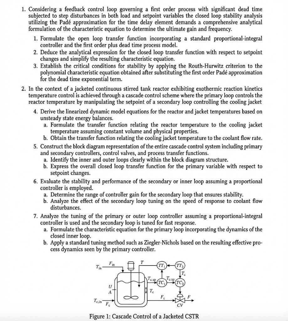 1. Considering a feedback control loop governing a first order process with significant dead time
subjected to step disturbances in both load and setpoint variables the closed loop stability analysis
utilizing the Padé approximation for the time delay element demands a comprehensive analytical
formulation of the characteristic equation to determine the ultimate gain and frequency.
1. Formulate the open loop transfer function incorporating a standard proportional-integral
controller and the first order plus dead time process model.
2. Deduce the analytical expression for the closed loop transfer function with respect to setpoint
changes and simplify the resulting characteristic equation.
3. Establish the critical conditions for stability by applying the Routh-Hurwitz criterion to the
polynomial characteristic equation obtained after substituting the first order Padé approximation
for the dead time exponential term.
2. In the context of a jacketed continuous stirred tank reactor exhibiting exothermic reaction kinetics
temperature control is achieved through a cascade control scheme where the primary loop controls the
reactor temperature by manipulating the setpoint of a secondary loop controlling the cooling jacket
4. Derive the linearized dynamic model equations for the reactor and jacket temperatures based on
unsteady state energy balances.
a. Formulate the transfer function relating the reactor temperature to the cooling jacket
temperature assuming constant volume and physical properties.
b. Obtain the transfer function relating the cooling jacket temperature to the coolant flow rate.
5. Construct the block diagram representation of the entire cascade control system including primary
and secondary controllers, control valves, and process transfer functions.
a. Identify the inner and outer loops clearly within the block diagram structure.
b. Express the overall closed loop transfer function for the primary variable with respect to
setpoint changes.
6. Evaluate the stability and performance of the secondary or inner loop assuming a proportional
controller is employed.
a. Determine the range of controller gain for the secondary loop that ensures stability.
b. Analyze the effect of the secondary loop tuning on the speed of response to coolant flow
disturbances.
7. Analyze the tuning of the primary or outer loop controller assuming a proportional-integral
controller is used and the secondary loop is tuned for fast response.
a. Formulate the characteristic equation for the primary loop incorporating the dynamics of the
closed inner loop.
b. Apply a standard tuning method such as Ziegler-Nichols based on the resulting effective pro-
cess dynamics seen by the primary controller.
ye 8 s (mm)
ea
(EN ely
A
TI CXD 4 F
al ow
Figure 1: Cascade Control of a Jacketed CSTR
Asked by: Francis
Created at: 2026-03-03 11:54:14
Final Answer:
📢 Instructions:
- Ask anything relatd to above question only.
- For new Question goto :