This is AI generated Response.
Asked by: Francis
Created at: 2026-02-25 08:27:34
Final Answer:
RenderedRaw Text
Did you like this answer?
Certainly! Let's walk through the step-by-step solution and explanation for deriving the Hamilton-Jacobi-Bellman (HJB) equation for the continuous-time optimal control problem described:
---
### **Step 1: Formulate the Dynamic Constraint Differential Equation**
The evolution of the system's state vector \( x(t) \) is governed by the differential equation:
\[
\dot{x}(t) = f(x(t), u(t), t)
\]
where \( u(t) \) is the control input.
---
### **Step 2: Express the Cost Functional**
The cost functional \( J \) to be minimized typically takes the form:
\[
J = \int_{t_}^{t_f} L(x(t), u(t), t) \, dt + K(x(t_f), t_f)
\]
where \( L \) is the running cost and \( K \) is the terminal cost.
---
### **Step 3: Define the Value Function**
The value function \( V(x, t) \) is defined as the minimum cost-to-go starting from state \( x \) at time \( t \):
\[
V(x, t) = \min_{u(\cdot)} \left[ \int_{t}^{t_f} L(x(\tau), u(\tau), \tau) \, d\tau + K(x(t_f), t_f) \right]
\]
where the minimization is taken over all admissible control trajectories.
---
### **Step 4: Apply the Principle of Optimality**
According to Bellman's principle of optimality, the value function at time \( t \) can be decomposed as:
\[
V(x, t) = \min_{u(\cdot)} \left[ \int_{t}^{t+\Delta t} L(x(\tau), u(\tau), \tau) d\tau + V(x(t+\Delta t), t+\Delta t) \right]
\]
For small \( \Delta t \), the first term approximates \( L(x, u, t)\Delta t \).
---
### **Step 5: Taylor Expansion of the Value Function**
Expand \( V(x(t+\Delta t), t+\Delta t) \) using a first-order Taylor series:
\[
V(x + \Delta x, t + \Delta t) \approx V(x, t) + \frac{\partial V}{\partial t} \Delta t + \nabla_x V \cdot \Delta x
\]
where \( \Delta x = f(x, u, t) \Delta t \).
---
### **Step 6: Substitute and Simplify**
Substitute the Taylor expansion into the optimality equation:
\[
V(x, t) = \min_{u} \left[ L(x, u, t) \Delta t + V(x, t) + \frac{\partial V}{\partial t} \Delta t + \nabla_x V \cdot f(x, u, t) \Delta t \right]
\]
Subtract \( V(x, t) \) from both sides and divide by \( \Delta t \):
\[
= \min_{u} \left[ L(x, u, t) + \frac{\partial V}{\partial t} + \nabla_x V \cdot f(x, u, t) \right]
\]
---
### **Step 7: Take the Limit as \( \Delta t \to \)**
As \( \Delta t \to \), you obtain the Hamilton-Jacobi-Bellman (HJB) partial differential equation:
\[
- \frac{\partial V}{\partial t} = \min_{u} \left[ L(x, u, t) + \nabla_x V \cdot f(x, u, t) \right]
\]
or equivalently,
\[
\frac{\partial V}{\partial t} + \min_{u} \left[ L(x, u, t) + \nabla_x V \cdot f(x, u, t) \right] =
\]
---
### **Step 8: Define the Hamiltonian**
Define the Hamiltonian function as:
\[
H(x, u, \nabla_x V, t) = L(x, u, t) + \nabla_x V \cdot f(x, u, t)
\]
So, the HJB equation becomes:
\[
\frac{\partial V}{\partial t} + \min_{u} H(x, u, \nabla_x V, t) =
\]
---
### **Step 9: Specify the Boundary Condition**
At the terminal time \( t_f \), the value function equals the terminal cost:
\[
V(x, t_f) = K(x, t_f)
\]
---
### **Step 10: Summary and Significance**
The HJB equation provides a necessary condition for optimality in continuous-time control problems. Solving this partial differential equation with the specified terminal boundary condition yields the optimal value function. The optimal control can then be obtained by choosing \( u \) at each state and time to minimize the Hamiltonian.
---
**Final Answer:**
The Hamilton-Jacobi-Bellman (HJB) equation for this continuous-time optimal control problem is:
\[
\boxed{
\frac{\partial V}{\partial t} + \min_{u} \left[ L(x, u, t) + \nabla_x V \cdot f(x, u, t) \right] =
}
\]
with the boundary condition:
\[
V(x, t_f) = K(x, t_f)
\]
This equation characterizes the optimal cost-to-go function and is central to dynamic programming approaches in optimal control.
Question:
Give me answer without empty values. and answer must be like student written type without using bullet-points.
This is AI generated Response.
Asked by: Francis
Created at: 2026-02-25 08:31:31
Final Answer:
RenderedRaw Text
Did you like this answer?
Certainly! Let’s go through the steps of deriving the Hamilton-Jacobi-Bellman (HJB) equation for the continuous-time optimal control problem in a student-friendly manner.
### Step 1: Formulate the Dynamic Constraint Differential Equation
The state evolution of the system is captured by the differential equation. It is expressed as \( \dot{x}(t) = f(x(t), u(t), t) \), where \( x(t) \) represents the state vector and \( u(t) \) is the control input.
### Step 2: Express the Cost Functional
To minimize the cost functional, we define it as \( J = \int_{t_0}^{t_f} L(x(t), u(t), t) \, dt + K(x(t_f), t_f) \). Here, \( L \) signifies the running cost incurred during the trajectory, while \( K \) indicates the terminal cost at the final time \( t_f \).
### Step 3: Define the Value Function
The value function, denoted as \( V(x, t) \), represents the minimum cost-to-go from the current state \( x \) at time \( t \). It is formulated as \( V(x, t) = \min_{u(\cdot)} \left[ \int_{t}^{t_f} L(x(\tau), u(\tau), \tau) \, d\tau + K(x(t_f), t_f) \right] \). The minimization is taken over all possible control trajectories.
### Step 4: Apply the Principle of Optimality
According to Bellman's principle, the value function can be decomposed as follows: \( V(x, t) = \min_{u(\cdot)} \left[ \int_{t}^{t+\Delta t} L(x(\tau), u(\tau), \tau) d\tau + V(x(t+\Delta t), t+\Delta t) \right] \). For a small increment \( \Delta t \), the first term approximates to \( L(x, u, t) \Delta t \).
### Step 5: Taylor Expansion of the Value Function
Next, we expand \( V(x(t+\Delta t), t+\Delta t) \) using a first-order Taylor series, which gives us \( V(x + \Delta x, t + \Delta t) \approx V(x, t) + \frac{\partial V}{\partial t} \Delta t + \nabla_x V \cdot \Delta x \). In this expression, \( \Delta x \) is equal to \( f(x, u, t) \Delta t \).
### Step 6: Substitute and Simplify
By substituting the Taylor series expansion into the optimality equation, we derive \( V(x, t) = \min_{u} \left[ L(x, u, t) \Delta t + V(x, t) + \frac{\partial V}{\partial t} \Delta t + \nabla_x V \cdot f(x, u, t) \Delta t \right] \). After subtracting \( V(x, t) \) and dividing by \( \Delta t \), we get \( 0 = \min_{u} \left[ L(x, u, t) + \frac{\partial V}{\partial t} + \nabla_x V \cdot f(x, u, t) \right] \).
### Step 7: Take the Limit as \( \Delta t \to 0 \)
Taking the limit as \( \Delta t \) approaches zero leads us to the HJB partial differential equation, expressed as \( - \frac{\partial V}{\partial t} = \min_{u} \left[ L(x, u, t) + \nabla_x V \cdot f(x, u, t) \right] \).
### Step 8: Define the Hamiltonian
We define the Hamiltonian function as \( H(x, u, \nabla_x V, t) = L(x, u, t) + \nabla_x V \cdot f(x, u, t) \). Thus, the HJB equation can be rewritten as \( \frac{\partial V}{\partial t} + \min_{u} H(x, u, \nabla_x V, t) = 0 \).
### Step 9: Specify the Boundary Condition
At the terminal time \( t_f \), we specify the boundary condition as \( V(x, t_f) = K(x, t_f) \). This condition helps to ensure that the value function matches the terminal cost.
### Step 10: Summary and Significance
The HJB equation we derived is critical for solving continuous-time optimal control problems. It characterizes the necessary conditions for optimality in terms of the value function. The unique solution to this equation, along with the boundary condition, allows us to determine the optimal control strategy by minimizing the Hamiltonian.
In conclusion, the HJB equation is given by:
\[
\frac{\partial V}{\partial t} + \min_{u} \left[ L(x, u, t) + \nabla_x V \cdot f(x, u, t) \right] = 0
\]
with the boundary condition:
\[
V(x, t_f) = K(x, t_f)
\]
This equation encapsulates the essence of dynamic programming in optimal control.
VIPSolutions focuses on clear, step‑by‑step explanations so you can learn quickly. Whether you need an AI‑generated walkthrough or a short hint to get unstuck, each solution is organized for fast reading and easy review later.
Search similar questions, compare approaches, and bookmark the best answers for revision. Our goal is simple: quick, reliable study help that feels natural—not noisy.
 VIPSolutions
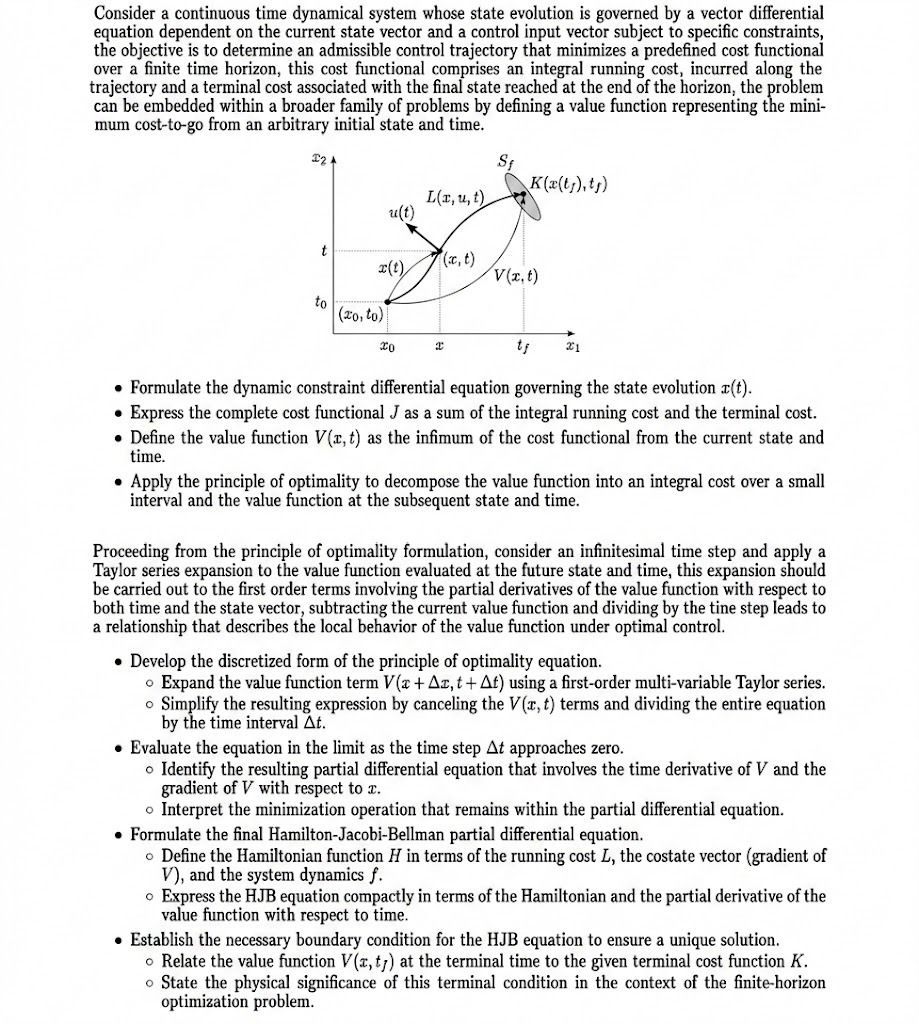 Consider a continuous time dynamical system whose state evolution is governed by a vector differential
equation dependent on the current state vector and a control input vector subject to specific constraints,
the objective is to determine an admissible control trajectory that minimizes a predefined cost functional
over a finite time horizon, this cost functional comprises an integral running cost, incurred along the
trajectory and a terminal cost associated with the final state reached at the end of the horizon, the pion
can be embedded within a broader family of problems by defining a value function representing the mini-
mum cost-to-go from an arbitrary initial state and time.
EA Sf
Ka(ty)t,
Hout) (e(tr)ty)
lt)
t
(et)
=) “4 fe €)
n 1
®| (oto)
ENE ty =
« Formulate the dynamic constraint differential equation governing the state evolution z(t).
© Express the complete cost functional J as a sum of the integral running cost and the terminal cost.
« Define the value function V(z,t) as the infimum of the cost functional from the current state and
time.
« Apply the principle of optimality to decompose the value function into an integral cost over a small
interval and the value function at the subsequent state and time.
Proceeding from the principle of optimality formulation, consider an infinitesimal time step and apply a
Taylor series expansion to the value function evaluated at the future state and time, this expansion should
be carried out to the first order terms involving the partial derivatives of the value function with respect to
both time and the state vector, subtracting the current value function and dividing by the tine step leads to
a relationship that describes the local behavior of the value function under optimal control.
« Develop the discretized form of the principle of optimality equation.
© Expand the value function term V(z + Az, t + Af) using a first-order multi-variable Taylor series.
o Simplify the resulting expression by canceling the V(x, f) terms and dividing the entire equation
by the time interval At.
« Evaluate the equation in the limit as the time step At approaches zero.
© Identify the resulting partial differential equation that involves the time derivative of V' and the
gradient of V with respect to .
o Interpret the minimization operation that remains within the partial differential equation.
« Formulate the final Hamilton-Jacobi-Bellman partial differential equation.
© Define the Hamiltonian function H in terms of the running cost L, the costate vector (gradient of
V), and the system dynamics f.
© Express the HLJB equation compactly in terms of the Hamiltonian and the partial derivative of the
value function with respect to time.
© Establish the necessary boundary condition for the HIB equation to ensure a unique solution.
© Relate the value function Vz, ;) at the terminal time to the given terminal cost function K.
© State the physical significance of this terminal condition in the context of the finite-horizon
optimization problem.