 VIPSolutions
Act like a helpful tutor and exlain me :P3.33 The attitude dynamics of a rocket are represented by Y(s) 1 —=G(s)=—, U(s) (s) 52 and state variable feedback is used where x11) = y(t), x(0) = $(0). and u() = a) Determine the roots of the characteristic equation of this system and the response of the system when the initial conditions are x;(0)=0 and x,(0)=1. The input U(s) is the applied torques, and Y(s) is the rocket attitude. Please Graph using Matlab
Question:
Act like a helpful tutor and exlain me :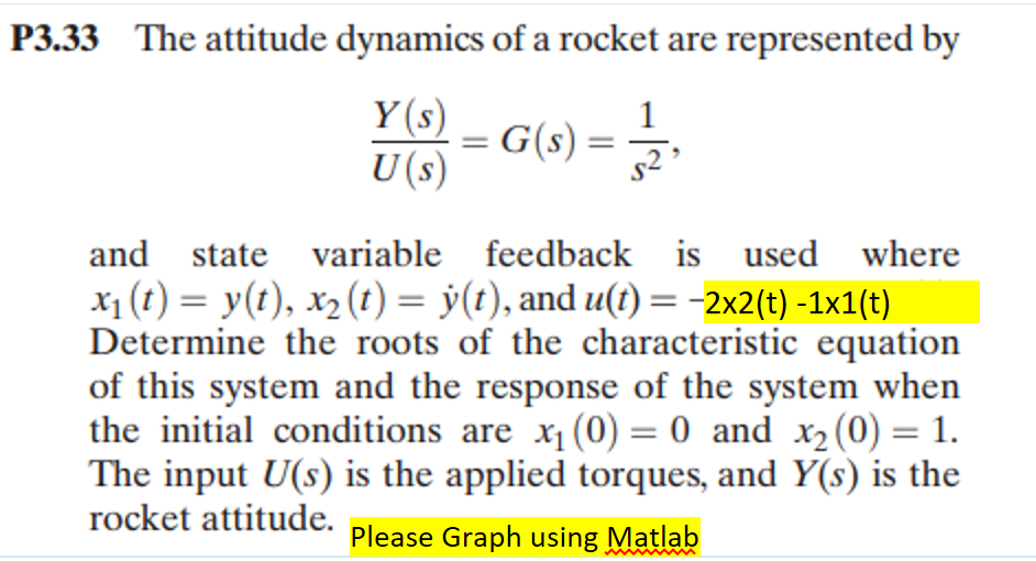 P3.33 The attitude dynamics of a rocket are represented by
Y(s) 1
—=G(s)=—,
U(s) (s) 52
and state variable feedback is used where
x11) = y(t), x(0) = $(0). and u() = a)
Determine the roots of the characteristic equation
of this system and the response of the system when
the initial conditions are x;(0)=0 and x,(0)=1.
The input U(s) is the applied torques, and Y(s) is the
rocket attitude. Please Graph using Matlab
This is AI generated Response.
Asked by: Alok Kumar
Created at: 2026-01-26 04:10:14
Asked by: Alok Kumar
Created at: 2026-01-26 04:10:14
Final Answer:
Rendered
Raw Text
Did you like this answer?
Let's break down and **solve** the problem step by step, then I'll show you how to **graph the in MATLAB**.
---
## **1. State-S Representation**
Given transfer function:
\[
\frac{Y(s)}{U(s)} =frac{1s^2}
\]
This is a **double integrator**.
Let:
- \( x_1(t) = y(t) \) (output/attitude)
- \( x_2(t) = \dot{y}(t) \) (angular velocity)
So,
\[
\dot{x}_1 = x_2
\]
\[
\dot{x}_2 = u(t)
\]
---
**2. State Feedback Law**
Given feedback:
\[
u(t) = -2x_2(t) - x_1(t)
\]
Substitute into state equations:
\[
\dot{x}_1 = x_2
\]
\[
\dot{x}_2 = -2x_2 - x_1
\]
Or, in matrix form:
\[
\begin{bmatrix}
\dot{x}_1 \\
\dot{x}_2
\end{bmatrix}
=
\begin{bmatrix}
& 1 \\
-1 & -2
\end{bmatrix}
\begin{bmatrix}
x_1 \\
x_2
\end{bmatrix}
\]
---
## **3. Characteristic Equation and Roots**
The system matrix \( A \) is:
\[
A = \begin{bmatrix}
& 1 \\
-1 & -2
\end{bmatrix}
\]
The characteristic equation:
\[
\det(sI - A) = \left| \begin{matrix}
s & -1 \\
1 & s+2
\end{matrix} \right| = s(s+2) + 1 = s^2 + 2s + 1 = (s+1)^2
\]
So the **roots** are:
\[
s = -1, -1
\]
(Double pole at -1)
---
## **4. Initial Conditions**
\[
x_1() = ,\quad x_2() = 1
\]
---
## **5. MATLAB Code for Response**
Let's simulate and plot \( x_1(t) \) and \( x_2(t) \):
```matlab
% State-space matrices
A = [ 1; -1 -2];
B = [; ]; % No external input, closed-loop
C = eye(2); % To get both x1 and x2
D = [; ];
% Initial conditions
x = [; 1];
% Time vector
t = linspace(, 10, 100);
% Simulate response
[y, t, x] = initial(ss(A, B, C, D), x, t);
% Plot
figure;
plot(t, x(:,1), 'b-', 'LineWidth', 2); hold on;
plot(t, x(:,2), 'r--', 'LineWidth', 2);
legend('x_1(t) = y(t) (Attitude)', 'x_2(t) = \dot{y}(t) (Rate)');
xlabel('Time (s)');
ylabel('States');
title('Rocket Attitude State Response');
grid on;
```
---
## **6. Explanation of the Code**
- **A**: system matrix from state-feedback closed loop.
- **x**: initial states.
- **initial**: MATLAB function to simulate the response of a state-space model.
- **Plot**: Shows both attitude and rate over time.
---
### **Summary Table**
| Step | Action | Result |
|------|---------------------|-------------------------------|
| 1 | State-space form | \(A = \begin{bmatrix} & 1\\-1 & -2\end{bmatrix}\) |
| 2 | Characteristic Eq. | \((s + 1)^2\) |
| 3 | Roots | \(s = -1, -1\) |
| 4 | Initial conditions | \(x_1()=,\ x_2()=1\) |
| 5 | MATLAB plot | See code above |
---
If you run this MATLAB code, you'll see the **system response** (attitude and rate) starting from your specified initial conditions! If you need further explanation or have questions about the state-space math or MATLAB code, just ask.
📢 Instructions:
- Ask anything relatd to above question only.
- For new Question goto :