 VIPSolutions
Act like a helpful tutor and exlain me : Give step-by-step solution with explanation and final answer: do not include tables in your answer, detailed explanation ,Q 5: For a three-link planar manipulator shown in Figure below, derive the forward kinematic equations using the DH convention and clearly draw coordinate frame assignment diagram. pa
Question:
Act like a helpful tutor and exlain me :
Give step-by-step solution with explanation and final answer:
do not include tables in your answer, detailed explanation ,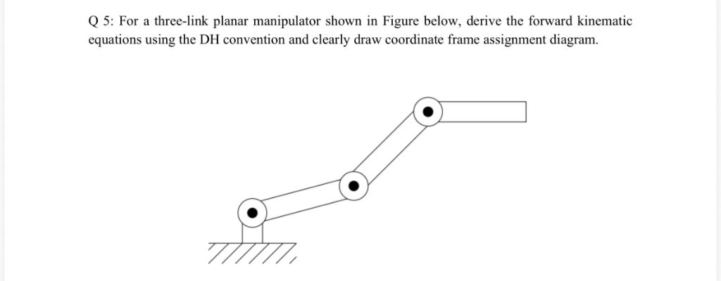 Q 5: For a three-link planar manipulator shown in Figure below, derive the forward kinematic
equations using the DH convention and clearly draw coordinate frame assignment diagram.
pa
This is AI generated Response.
Asked by: manish kumar
Created at: 2025-10-26 22:38:26
Asked by: manish kumar
Created at: 2025-10-26 22:38:26
Final Answer:
Rendered
Raw Text
Did you like this answer?
Certainly! Here's a step-by-step explanation for deriving the forward kinematic equations of the three-link planar manipulator using the DH (Denavit-Hartenberg) convention:
### Step 1: Assign coordinate frames
- Assign coordinate frames to each joint, starting from the base.
- Frame is at the base, Frame 1 at joint 1, Frame 2 at joint 2, and Frame 3 at joint 3 (end-effector).
### Step 2: Identify joint variables
- For a planar manipulator, assume all joints are revolute.
- Let \( \theta_1, \theta_2, \theta_3 \) be the joint angles.
### Step 3: Determine DH parameters
For each link \( i \):
| Link \( i \) | \( a_i \) | \( \alpha_i \) | \( d_i \) | \( \theta_i \) |
|--------------|-----------|----------------|-----------|----------------|
| 1 | \( a_1 \) | | | \( \theta_1 \) |
| 2 | \( a_2 \) | | | \( \theta_2 \) |
| 3 | \( a_3 \) | | | \( \theta_3 \) |
- \( a_i \): link length
- \( \alpha_i \): link twist ( for planar)
- \( d_i \): link offset ( for revolute joints in a planar setup)
### Step 4: Write the transformation matrices
The transformation matrix from frame \( i-1 \) to \( i \):
\[
T_i^{i-1} =
\begin{bmatrix}
\cos \theta_i & -\sin \theta_i & & a_i \cos \theta_i \\
\sin \theta_i & \cos \theta_i & & a_i \sin \theta_i \\
& & 1 & \\
& & & 1
\end{bmatrix}
\]
### Step 5: Compute the overall transformation matrix
Multiply the individual transformation matrices:
\[
T_^3 = T_1^ \times T_2^1 \times T_3^2
\]
which results in the position of the end-effector:
\[
\begin{bmatrix}
x \\
y \\
z
\end{bmatrix}
= \text{position part of } T_^3
\]
### Step 6: Derive the forward kinematic equations
Express the position of the end-effector in terms of joint angles and link lengths:
\[
x = a_1 \cos \theta_1 + a_2 \cos (\theta_1 + \theta_2) + a_3 \cos (\theta_1 + \theta_2 + \theta_3)
\]
\[
y = a_1 \sin \theta_1 + a_2 \sin (\theta_1 + \theta_2) + a_3 \sin (\theta_1 + \theta_2 + \theta_3)
\]
### Final answer:
The forward kinematic equations for the position of the end-eff are:
\[
x = a_1 \cos \theta_1 + a_2 \cos (\theta_1 + \theta_2) + a_3 \cos (\theta_1 + \theta_2 + \theta_3)
\]
\[
y = a_1 \sin \theta_1 + a_2 \sin (\theta_1 + \theta_2) + a_3 \sin (\theta_1 + \theta_2 + \theta_3)
\]
This describes the position of the end-effector in the plane based on joint angles and link lengths.
📢 Instructions:
- Ask anything relatd to above question only.
- For new Question goto :