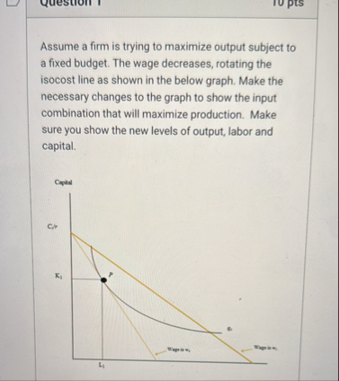
## Explanation of the Problem Let's break it down step by step! ### 1. **What is Given?** - A firm wants to **maximize output** given a **fixed budget**. - The **wage decreases** (cost of labor goes down). - The **isocost line** rotates (it gets flatter since labor is cheaper). - Graph has **capital (K)** on the y-axis and **labor (L)** on the x-axis. - The isocost lines for two wages (\(w_\) and \(w_1\), with \(w_1 < w_\)) are shown. - The original optimal point is \(P\), where the isocost is tangent to the isoquant (output curve). --- ### 2. **Graphical Representation** #### **Isocost Line** - Shows all combinations of capital and labor that cost the same total amount. - Equation: \[ \text{Budget} = wL + rK \] - When wage (\(w\)) decreases, the isocost line rotates outward (flatter), allowing more labor to be hired for the same budget. #### **Isoquant** - Curve showing combinations of labor and capital that produce the **same output**. --- ### 3. **How to Show the Change?** #### **Step 1: Draw the New Tangency** - **Find the new tangency point** between the new (flatter) isocost line and the highest possible isoquant. - This point will show the **new optimal combination** of labor and capital. #### **Step 2: Indicate the Changes** - **Output:** The firm can now reach a **higher isoquant** (higher output) because labor is cheaper. - **Labor:** The use of labor **increases** (move right on L-axis). - **Capital:** The use of capital could **increase, decrease, or stay the same** depending on the firm's production function, but usually, it decreases or stays similar as the firm substitutes cheaper labor for capital. --- ### 4. **How to Mark on the Graph** #### **Original Point (\(P\)):** - Tangency between old isocost and isoquant. #### **New Point (\(Q\)):** - Tangency between **new isocost line** (wage at \(w_1\)) and a **higher isoquant**. - Mark this new point as \(Q\). #### **Label the New Levels:** - **\(L_2\):** New higher labor level (project down to L-axis). - **\(K_2\):** New capital level (project across to K-axis). - **Higher Isoquant:** Draw and label the higher isoquant passing through \(Q\). --- ### 5. **Summary Table** | Before (Old Wage \(w_\)) | After (New Wage \(w_1\)) | |---------------------------|--------------------------| | Optimal at Point \(P\) | Optimal at Point \(Q\) | | Isoquant at initial output| Isoquant at higher output| | Labor = \(L_1\) | Labor = \(L_2 > L_1\) | | Capital = \(K_1\) | Capital = \(K_2\) | --- ## **How to Draw the Changes** 1. **Draw a new isoquant** above the original one to represent higher output. 2. **Find the tangency** between the new isocost (wage = \(w_1\)) and this new isoquant. 3. **Mark this point as \(Q\)**. 4. **Label the new labor and capital levels** (\(L_2, K_2\)) at \(Q\). --- ## **Key Takeaways** - **Decreased wage** → **Flatter isocost** → **More labor used**. - **Firm moves to higher output** (higher isoquant). - **Mark the new tangency and label the variables.** --- **If you want, I can sketch the modified graph for you as well!** Let me know if you'd like to see that.

# Explanation of the Problem Let's break it down step by step! ## 1. What is Given? - A firm aims to **maximize output** within a **fixed budget**. - The **wage decreases**, which means the cost of labor is lower. - The **isocost line** rotates, becoming flatter since labor is cheaper. - The graph has **capital (K)** on the y-axis and **labor (L)** on the x-axis. - The initial optimal point is \(P\), where the isocost is tangent to the isoquant (output curve). --- ## 2. Graphical Representation ### Isocost Line - Represents all combinations of capital and labor that cost the same total amount. - Equation: \[ \text{Budget} = wL + rK \] - A decrease in wage (\(w\)) causes the isocost line to rotate outward (flatter), allowing more labor to be hired within the same budget. ### Isoquant - A curve that shows combinations of labor and capital producing the **same output**. --- ## 3. How to Show the Change ### Step 1: Draw the New Tangency - Identify the new tangency point between the new (flatter) isocost line and the highest possible isoquant. - This point indicates the **new optimal combination** of labor and capital. ### Step 2: Indicate the Changes - **Output:** The firm can now reach a **higher isoquant** (higher output) since labor is cheaper. - **Labor:** The amount of labor **increases** (move right on the L-axis). - **Capital:** The use of capital may **increase, decrease, or remain the same** depending on the production function, but typically, it decreases or stays similar as the firm substitutes cheaper labor for capital. --- ## 4. How to Mark on the Graph ### Original Point (\(P\)) - The point of tangency between the old isocost and isoquant. ### New Point (\(Q\)) - The tangency between the **new isocost line** (with wage \(w_1\)) and a **higher isoquant**. - Label this new point as \(Q\). ### Label the New Levels - **\(L_2\)**: New higher labor level (project down to the L-axis). - **\(K_2\)**: New capital level (project across to the K-axis). - **Higher Isoquant**: Draw and label the higher isoquant passing through \(Q\). --- ## 5. Summary of Changes - **Before (Old Wage \(w_\))**: Optimal at Point \(P\), Isoquant at initial output, Labor = \(L_1\), Capital = \(K_1\). - **After (New Wage \(w_1\))**: Optimal at Point \(Q\), Isoquant at higher output, Labor = \(L_2 > L_1\), Capital = \(K_2\). --- ## Key Takeaways - A **decreased wage** leads to a **flatter isocost line**, resulting in **more labor usage**. - The firm moves to a **higher output** (higher isoquant). - Ensure to mark the new tangency and label the variables clearly. --- If you need a visual representation of the modified graph, let me know!

# Summary of Changes in Input Combination for Maximal Production ## Overview A firm is maximizing output with a fixed budget, and a decrease in wages has occurred. This change affects the isocost line, which represents the combinations of labor and capital that can be purchased for a given budget. ## Key Changes - **Isocost Line:** The line rotates outward (flatter) due to the decrease in the wage rate, allowing more labor to be hired for the same budget. - **Isoquant:** Indicates combinations of labor and capital that yield the same output. With the new isocost, the firm can reach a higher isoquant. ## Input Levels - **Original Optimal Point:** At point \(P\), where the old isocost line touches the isoquant. - **New Optimal Point:** At point \(Q\), where the new isocost line is tangent to a higher isoquant. - **Labor (L):** Increases from \(L_1\) to \(L_2\) due to cheaper labor. - **Capital (K):** May either decrease, increase, or remain the same, but typically decreases as firms substitute labor for capital. ## Conclusion The overall effect of the wage decrease is an increase in labor usage and a potential increase in output, as represented by the movement to a higher isoquant. The new input combination is marked at point \(Q\), reflecting the optimal mix of labor and capital under the new wage conditions.

To calculate the concentration of CO in mg/m³, we can follow these steps: ### Step 1: Calculate the Molar Volume at 25°C and 1 atm Using the ideal gas law, the molar volume at standard conditions (0°C and 1 atm) is approximately 22.4 L. However, at 25°C, the molar volume can be approximated using the ideal gas law: \[ V_m = \frac{RT}{P} \] Where: - \( R \) = 0.0821 L·atm/(K·mol) (ideal gas constant) - \( T \) = 25°C = 298 K - \( P \) = 1 atm \[ V_m = \frac{(0.0821 \, \text{L·atm/(K·mol)}) \times (298 \, \text{K})}{1 \, \text{atm}} \approx 24.45 \, \text{L/mol} \] ### Step 2: Convert Molar Volume to Cubic Meters \[ V_m = 24.45 \, \text{L/mol} = 24.45 \times 10^{-3} \, \text{m}^3/\text{mol} \] ### Step 3: Calculate the Volume Fraction of CO The volume fraction of CO is given as 4.4%, which means: \[ \text{Volume of CO} = 0.044 \times V_m \] ### Step 4: Calculate Number of Moles of CO in 1 m³ To find the number of moles of CO in 1 m³: \[ n = \frac{1 \, \text{m}^3}{V_m} \, \text{mol} \] \[ n = \frac{1}{24.45 \times 10^{-3}} \approx 40.9 \, \text{mol} \] ### Step 5: Calculate Moles of CO Using the volume fraction: \[ n_{CO} = 0.044 \times 40.9 \approx 1.8 \, \text{mol} \] ### Step 6: Convert Moles of CO to Grams Using the molar mass of CO (28 g/mol): \[ \text{Mass of CO} = n_{CO} \times \text{Molar Mass} = 1.8 \, \text{mol} \times 28 \, \text{g/mol} \approx 50.4 \, \text{g} \] ### Step 7: Convert Grams to Milligrams \[ \text{Mass in mg} = 50.4 \, \text{g} \times 1000 = 50400 \, \text{mg} \] ### Step 8: Calculate the Concentration in mg/m³ The concentration of CO in the air is therefore: \[ \text{Concentration of CO} = 50400 \, \text{mg/m}^3 \] ### Final Answer The concentration of CO in mg/m³ is: \[ \boxed{50400} \]