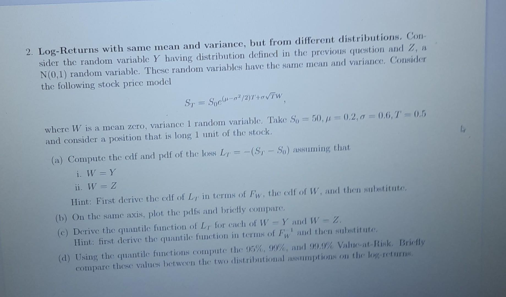
Act like a helpful tutor and exlain me :2. Tog-Returns with same mean and variance, but from different distributions. Con
cr tho random variable ¥ having distribution defined in the previous question and Z, i
N(0,1) random variable. These random variables have the same mean and variance, Consider
the following stock price model
Sp = Spelt [21h TW
where W is a mean zero, variance 1 random variable. Take Sy = 50, p= 02,0 = 0.6,1 = 0.5 4
and consider a position that is long 1 unit of the stock. oa
Ee (a) Compute the cdf and pdf of the Joss Ly = — (Sp — So) assuming that a
aw =Y a
- i w=2 a
‘Hint: First derive the cdf of Ly: in terms of Fy, tho cdf of W, and then substi
(b) On the same axis, plot the pdfs and Briefly compare, ,
Derive the quantile function of Ly: for cach of WW —Y and W = Z
at: first derive the quantile function in crm of Fy! and then su
tile fanctions compute the 95%, 99%
ales between the two distributional
Question:
Act like a helpful tutor and exlain me :2. Tog-Returns with same mean and variance, but from different distributions. Con
cr tho random variable ¥ having distribution defined in the previous question and Z, i
N(0,1) random variable. These random variables have the same mean and variance, Consider
the following stock price model
Sp = Spelt [21h TW
where W is a mean zero, variance 1 random variable. Take Sy = 50, p= 02,0 = 0.6,1 = 0.5 4
and consider a position that is long 1 unit of the stock. oa
Ee (a) Compute the cdf and pdf of the Joss Ly = — (Sp — So) assuming that a
aw =Y a
- i w=2 a
‘Hint: First derive the cdf of Ly: in terms of Fy, tho cdf of W, and then substi
(b) On the same axis, plot the pdfs and Briefly compare, ,
Derive the quantile function of Ly: for cach of WW —Y and W = Z
at: first derive the quantile function in crm of Fy! and then su
tile fanctions compute the 95%, 99%
ales between the two distributional
This is AI generated Response.
Asked by: Umesh
Created at: 2025-08-05 23:58:48
Final Answer:
RenderedRaw Text
Did you like this answer?
Absolutely! Let's break down the problem step by step:
---
**2. Log-Returns with same mean and variance, but from different distributions**
You’re given a stock price model:
\[
S_T = S_0 e^{(\mu - \sigma^2/2)T + \sigma \sqrt{T} W}
\]
where:
- \(W\) is a random variable with mean 0 and variance 1.
- You have two cases: \(W = Y\) (some distribution from the previous question) and \(W = Z\) (standard normal \(\mathcal{N}(0,1)\)).
- The parameters: \(S_0 = 50\), \(\mu = 0.2\), \(\sigma = 0.6\), \(T = 0.5\).
You consider a position that is long 1 unit of the stock, and you are interested in the **loss**:
\[
L_T = -(S_T - S_0) = S_0 - S_T
\]
Let's answer each part:
---
## (a) Compute the cdf and pdf of the loss \(L_T\) for both cases
**Hint:** Express \(L_T\) in terms of \(W\), then use the distribution of \(W\).
### Step 1: Express \(L_T\) in terms of \(W\)
\[
S_T = S_0 e^{(\mu - \sigma^2/2)T + \sigma \sqrt{T} W}
\]
\[
L_T = S_0 - S_T = S_0 - S_0 e^{(\mu - \sigma^2/2)T + \sigma \sqrt{T} W}
\]
\[
L_T = S_0 \left[1 - e^{(\mu - \sigma^2/2)T + \sigma \sqrt{T} W}\right]
\]
### Step 2: Find the cdf and pdf
Let \(X = (\mu - \sigma^2/2)T + \sigma \sqrt{T} W\). Then,
\[
L_T = S_0 (1 - e^X)
\]
Given \(W\), \(X\) is a monotonic function of \(W\).
#### CDF:
\[
F_{L_T}(l) = P(L_T \leq l) = P(S_0 (1 - e^X) \leq l)
\]
\[
\Rightarrow 1 - e^X \leq \frac{l}{S_0}
\]
\[
\Rightarrow e^X \geq 1 - \frac{l}{S_0}
\]
\[
\Rightarrow X \geq \ln\left(1 - \frac{l}{S_0}\right)
\]
Since \(X\) is a linear function of \(W\), for \(W = Y\) or \(Z\):
\[
X = (\mu - \sigma^2/2)T + \sigma\sqrt{T}W
\]
\[
W \geq \frac{\ln(1 - l/S_0) - (\mu - \sigma^2/2)T}{\sigma\sqrt{T}}
\]
Let’s call this threshold \(w^*\):
\[
w^* = \frac{\ln(1 - l/S_0) - (\mu - \sigma^2/2)T}{\sigma\sqrt{T}}
\]
So,
\[
F_{L_T}(l) = P(W \geq w^*)
\]
or
\[
F_{L_T}(l) = 1 - F_W(w^*)
\]
where \(F_W\) is the cdf of \(W\).
#### PDF:
\[
f_{L_T}(l) = \frac{d}{dl} F_{L_T}(l) = -f_W(w^*) \cdot \frac{d w^*}{dl}
\]
Compute the derivative:
\[
\frac{d w^*}{dl} = \frac{-1}{\sigma\sqrt{T}(1 - l/S_0) S_0}
\]
So,
\[
f_{L_T}(l) = f_W(w^*) \cdot \frac{1}{\sigma\sqrt{T}(1 - l/S_0) S_0}
\]
**In summary:**
- For both \(W = Y\) and \(W = Z\), use their respective cdf/pdf in the above formulas.
---
## (b) Plot the pdfs and compare
- On the same axis, plot the pdfs \(f_{L_T}(l)\) for \(W = Y\) and \(W = Z\).
- **Brief comparison:** The shape of the loss distributions will depend on the tail behavior of \(Y\) and \(Z\). If \(Y\) has heavier tails, the loss distribution will also have heavier tails, indicating higher probability of extreme losses.
---
## (c) Derive the quantile function of \(L_T\)
Quantile function: Given \(q\), find \(l_q\) such that \(P(L_T \leq l_q) = q\).
From above:
\[
F_{L_T}(l_q) = 1 - F_W(w^*) = q
\]
\[
F_W(w^*) = 1 - q
\]
\[
w^* = F_W^{-1}(1 - q)
\]
Recall:
\[
l_q = S_0 (1 - e^{(\mu-\sigma^2/2)T + \sigma\sqrt{T}w_q})
\]
where \(w_q = F_W^{-1}(1 - q)\).
---
## (d) Compute the Value-at-Risk (VaR) at 95%, 99%, and 99.9%
- **VaR at level \(q\):** This is just the quantile \(l_q\) for \(q = 0.95, 0.99, 0.999\).
- **Compare:** For heavier-tailed \(Y\), VaR will be larger at high confidence levels (e.g., 99%, 99.9%), reflecting larger potential for extreme losses.
---
### **Summary Table**
| Step | Formula |
|------|---------|
| Loss | \(L_T = S_0 (1 - e^{(\mu-\sigma^2/2)T + \sigma\sqrt{T}W})\) |
| CDF | \(F_{L_T}(l) = 1 - F_W(w^*)\), \(w^* = \frac{\ln(1 - l/S_0) - (\mu-\sigma^2/2)T}{\sigma\sqrt{T}}\) |
| PDF | \(f_{L_T}(l) = f_W(w^*) / [\sigma\sqrt{T} (1 - l/S_0) S_0]\) |
| Quantile | \(l_q = S_0 [1 - e^{(\mu-\sigma^2/2)T + \sigma\sqrt{T} w_q}]\), \(w_q = F_W^{-1}(1 - q)\) |
| VaR | \(VaR_q = l_q\) |
---
If you need help with plotting or coding, or the specifics about the distribution \(Y\), let me know!
VIPSolutions focuses on clear, step‑by‑step explanations so you can learn quickly. Whether you need an AI‑generated walkthrough or a short hint to get unstuck, each solution is organized for fast reading and easy review later.
Search similar questions, compare approaches, and bookmark the best answers for revision. Our goal is simple: quick, reliable study help that feels natural—not noisy.
 VIPSolutions
 2. Tog-Returns with same mean and variance, but from different distributions. Con
cr tho random variable ¥ having distribution defined in the previous question and Z, i
N(0,1) random variable. These random variables have the same mean and variance, Consider
the following stock price model
Sp = Spelt [21h TW
where W is a mean zero, variance 1 random variable. Take Sy = 50, p= 02,0 = 0.6,1 = 0.5 4
and consider a position that is long 1 unit of the stock. oa
Ee (a) Compute the cdf and pdf of the Joss Ly = — (Sp — So) assuming that a
aw =Y a
- i w=2 a
‘Hint: First derive the cdf of Ly: in terms of Fy, tho cdf of W, and then substi
(b) On the same axis, plot the pdfs and Briefly compare, ,
Derive the quantile function of Ly: for cach of WW —Y and W = Z
at: first derive the quantile function in crm of Fy! and then su
tile fanctions compute the 95%, 99%
ales between the two distributional