 VIPSolutions
Act like a helpful tutor and exlain me :1. State the nature of the following transfer functions (e.g, overdamped, underdamped, etc). Justify your answers by showing how you extract the relevaut information from the coeficients. @) 6) = sess (b) T(s) = llr (©) 706) = kms 2. For the system whose transfer function is 7-4. sketch the system response to step input, find the following values, and indicate them on the sketch (you may make more than one copy of the sketch if it makes things cleaner to draw) (8) The steady-state (ie. final) value (b) The 10-90% rise time {(¢) The 2% settling time (d) The maximum % overshoot For each of these quantities, show both your work and the numeric value of the answer to one deciuial place
Question:
Act like a helpful tutor and exlain me :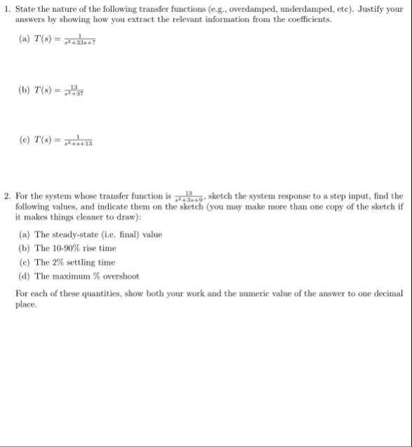 1. State the nature of the following transfer functions (e.g, overdamped, underdamped, etc). Justify your
answers by showing how you extract the relevaut information from the coeficients.
@) 6) = sess
(b) T(s) = llr
(©) 706) = kms
2. For the system whose transfer function is 7-4. sketch the system response to step input, find the
following values, and indicate them on the sketch (you may make more than one copy of the sketch if
it makes things cleaner to draw)
(8) The steady-state (ie. final) value
(b) The 10-90% rise time
{(¢) The 2% settling time
(d) The maximum % overshoot
For each of these quantities, show both your work and the numeric value of the answer to one deciuial
place
This is AI generated Response.
Asked by: Alok Kumar
Created at: 2026-02-03 05:23:24
Asked by: Alok Kumar
Created at: 2026-02-03 05:23:24
Final Answer:
Rendered
Raw Text
Did you like this answer?
Sure! Let's work through each part step-by-step.
---
# 1. **Nature of the Transfer Functions**
A standard second-order system has the form:
\[
T(s) = \frac{\omega_n^2}{s^2 + 2\zeta\omega_n s + \omega_n^2}
\]
where:
- \(\omega_n\) = natural frequency
- \(\zeta\) = damping ratio
The nature depends on \(\zeta\):
- **Overdamped:** \(\zeta > 1\)
- **Critically damped:** \(\zeta = 1\)
- **Underdamped:** \( < \zeta < 1\)
- **Undamped:** \(\zeta = \)
Let's analyze each transfer function:
---
### (a) \(T(s) = \frac{1}{s^2 + 3s + 7}\)
Compare to standard form:
- \(2\zeta\omega_n = 3\)
- \(\omega_n^2 = 7\) → \(\omega_n = \sqrt{7} \approx 2.65\)
So,
\[
2\zeta\omega_n = 3 \implies \zeta = \frac{3}{2\omega_n} = \frac{3}{2 \times 2.65} \approx .57
\]
**Conclusion**:
\(\zeta \approx .57\) (\( < \zeta < 1\)), so it is **underdamped**.
---
### (b) \(T(s) = \frac{13}{s^2 + 4s + 37}\)
- \(2\zeta\omega_n = 4\)
- \(\omega_n^2 = 37 \implies \omega_n = \sqrt{37} \approx 6.08\)
So,
\[
\zeta = \frac{4}{2 \times 6.08} \approx .33
\]
**Conclusion:**
\(\zeta \approx .33\) (\( < \zeta < 1\)), so it is **underdamped**.
---
### (c) \(T(s) = \frac{1}{s^2 + 4s + 13}\)
- \(2\zeta\omega_n = 4\)
- \(\omega_n^2 = 13 \implies \omega_n = \sqrt{13} \approx 3.61\)
So,
\[
\zeta = \frac{4}{2 \times 3.61} \approx .55
\]
**Conclusion:**
\(\zeta \approx .55\) (\( < \zeta < 1\)), so it is **underdamped**.
---
# 2. **Step Response Analysis for \(T(s) = \frac{13}{s^2 + 4s + 37}\)**
Let’s analyze for a unit step input:
## **a) Steady-State (Final) Value**
For a unit step input (\(R(s) = \frac{1}{s}\)), use the Final Value Theorem:
\[
y_{ss} = \lim_{t \to \infty} y(t) = \lim_{s \to } sY(s)
\]
\[
Y(s) = T(s) \cdot R(s) = \frac{13}{s^2 + 4s + 37} \cdot \frac{1}{s}
\]
\[
y_{ss} = \lim_{s \to } s \cdot \frac{13}{s(s^2 + 4s + 37)} = \frac{13}{37}
\]
\[
\approx .351
\]
---
## **b) 10-90% Rise Time**
Rise time (\(t_r\)) for underdamped system is approximately:
\[
t_r \approx \frac{\pi - \theta}{\omega_d}
\]
where
- \(\omega_d = \omega_n \sqrt{1-\zeta^2}\)
- \(\theta = \arccos(\zeta)\)
Given:
- \(\omega_n = 6.08\)
- \(\zeta = .33\)
Calculate:
- \(\omega_d = 6.08 \sqrt{1-.33^2} = 6.08 \times .944 = 5.74\)
- \(\theta = \arccos(.33) \approx 1.23\) radians
\[
t_r \approx \frac{\pi - 1.23}{5.74} = \frac{1.91}{5.74} \approx .33 \text{ s}
\]
---
## **c) 2% Settling Time**
Settling time (\(t_s\)):
\[
t_s \approx \frac{4}{\zeta \omega_n} = \frac{4}{.33 \times 6.08} = \frac{4}{2.01} \approx 2. \text{ s}
\]
---
## **d) Maximum % Overshoot**
\[
\%OS = e^{-\frac{\zeta \pi}{\sqrt{1-\zeta^2}}} \times 100\%
\]
\[
\sqrt{1-.33^2} \approx .944
\]
\[
-\frac{.33 \pi}{.944} \approx -1.097
\]
\[
\%OS = e^{-1.097} \times 100 \approx 33.4\%
\]
---
## **Summary Table**
| Quantity | Formula | Value |
|--------------|---------|---------|
| Steady-State | \(\frac{13}{37}\) | .4 |
| Rise Time | \(\frac{\pi - \arccos(\zeta)}{\omega_d}\) | .3 s |
| Settling Time| \(\frac{4}{\zeta\omega_n}\) | 2. s |
| % Overshoot | \(e^{-\frac{\zeta \pi}{\sqrt{1-\zeta^2}}} \times 100\%\) | 33.4% |
---
## **Sketch**
- The step response will rise quickly, overshoot by ~33%, and settle to .4 after about 2 seconds.
- Mark .4 on the y-axis, .3 s for rise time, 2. s for settling time, and the overshoot peak at ~.53.
---
**Let me know if you want a hand-drawn sketch or further clarifications!**
📢 Instructions:
- Ask anything relatd to above question only.
- For new Question goto :