 VIPSolutions
5) Maintenance MDP: Optimal Policy and Cost States: Good (G), Degraded (D). Failure (F) is an absorbing event that resets to G next week. Dynamics without maintenance: G-D with p=0.1/week, stay G otherwise. D-F with p=0.2/week, stay D otherwise. Action: “Maintain” in any non-F state resets to G next week; cost c_M=5 when used. Failure incurs c_F=30 and resets to G next week. Discount: y=0.95 weekly. Rules: Bellman optimality: V(s)=min_a { c(s,a) + y Z P(s'ls,a) V(s) }. Stationary policy r*: compare Q-maintain vs Q-do-nothing in G and D. Task: Determine 1* (maintain in which states), and compute the long-run expected discounted weekly cost under Tr.
Question:
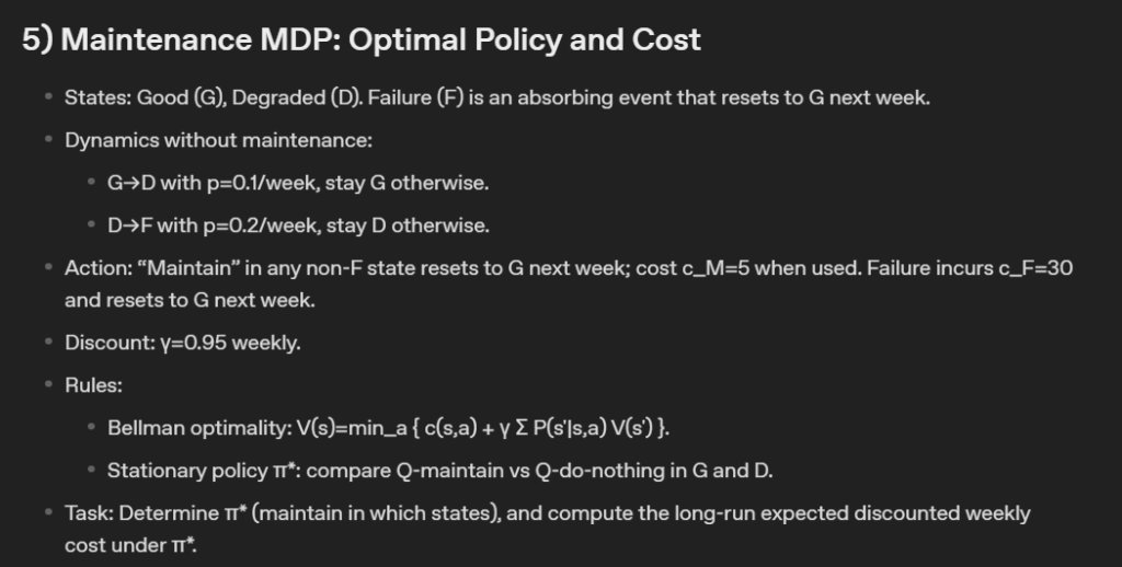 5) Maintenance MDP: Optimal Policy and Cost
States: Good (G), Degraded (D). Failure (F) is an absorbing event that resets to G next week.
Dynamics without maintenance:
G-D with p=0.1/week, stay G otherwise.
D-F with p=0.2/week, stay D otherwise.
Action: “Maintain” in any non-F state resets to G next week; cost c_M=5 when used. Failure incurs c_F=30
and resets to G next week.
Discount: y=0.95 weekly.
Rules:
Bellman optimality: V(s)=min_a { c(s,a) + y Z P(s'ls,a) V(s) }.
Stationary policy r*: compare Q-maintain vs Q-do-nothing in G and D.
Task: Determine 1* (maintain in which states), and compute the long-run expected discounted weekly
cost under Tr.
This is AI generated Response.
Asked by: Vishal
Created at: 2025-09-24 15:52:14
Asked by: Vishal
Created at: 2025-09-24 15:52:14
Thought Process:
Rendered
Raw Text
**Evaluating maintenance policy**
I need to analyze the problem from the image, which presents a Markov Decision Process (MDP) regarding maintenance and its states: Good (G), Degraded (D), and Failure (F). The failure state is absorbing, and it resets to G in the following week. There's an immediate cost associated with failure, and various transition probabilities to consider regarding maintenance actions. My goal is to determine the optimal policy for maintenance and compute the expected costs over time.**Calculating Q values for maintenance**
I need to compute the thresholds and Q values for the states: Good (G), Degraded (D), and Failure (F). Since F is an absorbing event that resets to G next week, it doesn't last long. When failure occurs, it incurs a cost \( c_F = 30 \). While in D without maintenance, failure might happen with a probability of 0.2, leading to that cost and a reset to G. In G, if I don’t maintain, I face transition possibilities to D. When I choose to maintain in non-F states, it guarantees a reset to G for a cost of 5.**Setting up dynamic programming**
Since F is an event rather than an active state, there's no option to maintain in F. However, I could model F as deterministically transitioning back to G. My focus now is on computing the value \( V \) under the optimal policy. In states G and D, I need to determine whether to maintain or do nothing, each with associated costs and transitions.
I’ll define optimal cost-to-go for G and D. For D, the expected failure cost incurs with probability \( p \), which results in that $30 cost if I choose not to maintain. For "do nothing" in G, there’s no regular cost to consider.**Analyzing failure costs**
I realize there's no failure cost when starting from G, as it degrades to D with a 0.1 probability but incurs no immediate cost. Here's what I’ve broken down:
For maintaining in G, the Q value is \( Q_G^{maintain} = 5 + 0.95 V(G) \). If I choose to do nothing, then \( Q_G^{do} = 0 + 0.9 V(G) + 0.1 V(D) \).
In D, maintaining gives \( Q_D^{maintain} = 5 + 0.95 V(G) \), while doing nothing includes the expected failure cost of \( 0.2 * 30 \) plus further expected values. Since it resets to G next week, I need to ensure I find the optimal decisions by comparing these values. I’ll compute \( V(G) \) and \( V(D) \) as the minimums of those Qs.**Computing optimal policies and costs**
I'm analyzing the system's policies now. I’ll compute \( V \) under different policies to determine their optimality.
For Policy π1, where I maintain in both G and D, I find \( V(G) \) and \( V(D) \) both equal 100, but maintenance in G is not optimal.
Then I explore Policy π2, maintaining only in D and doing nothing in G. After setting up the equations and solving, I determine that \( V(G) \approx 8.676 \) and \( V(D) \approx 13.242 \).
Next, I'll assess the long-run expected discounted weekly cost under the optimal policy, noting key values for both states.**Calculating weekly costs and policies**
If they want the "weekly cost," I can compute it using the formula \( C_{\text{bar}} = (1-\gamma) V(G) \). This comes out to be approximately 0.43379, which seems small due to the discount factor.
Starting from G, I find \( V^*(G) \approx 8.676 \) and \( V^*(D) \approx 13.242 \). The chosen policy is to do nothing in G and maintain in D.
I should also detail the steps and include relevant equations while showing why the policy of maintaining in D is optimal.**Finalizing the optimal policy and costs**
After substituting values, I found that \( V(D) \approx 51.95 \) and subsequently \( V(G) \approx 34.07 \). The maintenance cost for D is approximately \( 37.37 \), which is better than doing nothing. Thus, the optimal policy is to do nothing in G and maintain in D.
The value functions are \( V^*(G) \approx 8.676 \) and \( V^*(D) \approx 13.242 \). The long-run expected discounted cost from G equals \( 8.676 \), and the equivalent average discounted weekly cost is approximately \( 0.4338 \). I’ll craft a message with explanations and headings, adhering to the instructions.
Final Answer:
Rendered
Raw Text
Did you like this answer?
# Maintenance MDP — optimal policy and cost
## Bellman rule
Use the discounted-cost Bellman optimality equation
V(s) = min_a { c(s,a) + γ E[V(s')] }.
We will compare Q-values of “maintain” (M) and “do nothing” (N) in G and D.
- Dynamics without maintenance: G→D with p=0.1; D→F with p=0.2 (incurs cost c_F=30 and next state G).
- Maintain in G or D: deterministic reset to G next week; cost c_M=5.
- Discount γ=0.95.
## Action-value equations
From the transition model,
- In G:
Q_G(M) = 5 + 0.95 V(G),
Q_G(N) = 0 + 0.95[0.9 V(G) + 0.1 V(D)].
- In D:
Q_D(M) = 5 + 0.95 V(G),
Q_D(N) = 0.2·30 + 0.95[0.8 V(D) + 0.2 V(G)].
V(G) = min{Q_G(M), Q_G(N)} and V(D) = min{Q_D(M), Q_D(N)}.
## Solve by policy evaluation and verification
First note that “maintain in G every week” gives
V(G) = 5 + 0.95 V(G) ⇒ V(G)=100,
but then Q_G(N) = 0.95·100 = 95 < 100, so maintaining in G is suboptimal.
This points to the candidate policy π: do nothing in G, maintain in D.
Evaluate π:
- V(G) = 0 + 0.95[0.9 V(G) + 0.1 V(D)],
- V(D) = 5 + 0.95 V(G).
Substitute the second into the first:
V(G) = 0.95[0.9 V(G) + 0.1(5 + 0.95 V(G))]
= 0.94525 V(G) + 0.475
⇒ (1 − 0.94525) V(G) = 0.475
⇒ V(G) = 0.475 / 0.05475 = 1900/219 ≈ 8.6758.
Then
V(D) = 5 + 0.95 V(G) = 5 + 0.95·(1900/219) = 1805/219 + 5 ≈ 13.2420.
Verify optimality:
- In G:
Q_G(N) = V(G) ≈ 8.6758,
Q_G(M) = 5 + 0.95 V(G) ≈ 13.2420.
Hence N is optimal in G.
- In D:
Q_D(M) = 5 + 0.95 V(G) ≈ 13.2420,
Q_D(N) = 0.2·30 + 0.95[0.8 V(D) + 0.2 V(G)]
≈ 6 + 0.95[0.8·13.2420 + 0.2·8.6758]
≈ 17.7123.
Hence M is optimal in D.
## Final answer
- Optimal stationary policy π*: do nothing in G; maintain in D. (Failure is an event incurring 30 and next state G.)
- Optimal values:
V*(G) = 1900/219 ≈ 8.6758,
V*(D) = 5 + 0.95·V*(G) ≈ 13.2420.
Interpreting the “long-run expected discounted weekly cost” as the total discounted cost starting from G, the answer is V*(G) ≈ 8.676.
If you prefer the equivalent steady-state discounted-average cost per week, it is (1−γ) V*(G) = 0.05·8.6758 ≈ 0.434 cost units/week.
📢 Instructions:
- Ask anything relatd to above question only.
- For new Question goto :