w—y/
Plt) Cy A
m /
Xz Cz
7 us
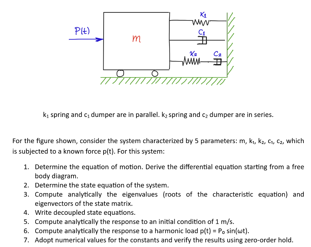
ky spring and c; dumper are in parallel. k; spring and c; dumper are in series.
For the figure shown, consider the system characterized by 5 parameters: m, ky, k, ¢;, cz, which
is subjected to a known force p(t). For this system:
1. Determine the equation of motion. Derive the differential equation starting from a free
body diagram.
2. Determine the state equation of the system.
3. Compute analytically the eigenvalues (roots of the characteristic equation) and
eigenvectors of the state matrix.
4. Write decoupled state equations.
5. Compute analytically the response to an initial condition of 1 m/s.
6. Compute analytically the response to a harmonic load p(t) = Po sin(wt).
7. Adopt numerical values for the constants and verify the results using zero-order hold.
Question:
w—y/
Plt) Cy A
m /
Xz Cz
7 us
ky spring and c; dumper are in parallel. k; spring and c; dumper are in series.
For the figure shown, consider the system characterized by 5 parameters: m, ky, k, ¢;, cz, which
is subjected to a known force p(t). For this system:
1. Determine the equation of motion. Derive the differential equation starting from a free
body diagram.
2. Determine the state equation of the system.
3. Compute analytically the eigenvalues (roots of the characteristic equation) and
eigenvectors of the state matrix.
4. Write decoupled state equations.
5. Compute analytically the response to an initial condition of 1 m/s.
6. Compute analytically the response to a harmonic load p(t) = Po sin(wt).
7. Adopt numerical values for the constants and verify the results using zero-order hold.
This is AI generated Response.
Asked by: Adapaka Jagadeesh
Created at: 2025-09-01 18:18:13
Final Answer:
RenderedRaw Text
Did you like this answer?
Let's break down the solution steps for the given mechanical system:
---
## **Step 1: Equation of Motion (Differential Equation)**
### **Free Body Diagram Analysis**
- **Mass \( m \):** Subjected to external force \( p(t) \).
- **Right Side:** Two parallel elements (\(k_1, c_1\)) in parallel with a series combination of \(k_2, c_2\).
#### **Equivalent Stiffness and Damping**
- **Parallel branch:** \(k_1, c_1\)
- **Series branch:** \(k_2\) and \(c_2\) in series
#### **Force on Mass:**
\[
m\ddot{x}(t) = p(t) - F_{\text{parallel}} - F_{\text{series}}
\]
#### **Parallel Branch:**
\[
F_{k_1+c_1} = k_1x + c_1\dot{x}
\]
#### **Series Branch (Spring-Damper in Series):**
Let \( z \) be the displacement at the node between \( k_2 \) and \( c_2 \).
- Force through both elements is the same: \( F_{series} \)
- Displacement across both: \( x \)
- \( x = x_{k_2} + x_{c_2} \)
- \( F_{k_2} = k_2(x - z) \)
- \( F_{c_2} = c_2(\dot{x} - \dot{z}) \)
- \( F_{k_2} = F_{c_2} = F_{series} \)
So,
\[
k_2(x-z) = c_2(\dot{x} - \dot{z})
\]
\[
\Rightarrow k_2(x-z) = c_2(\dot{x} - \dot{z})
\]
\[
\Rightarrow k_2(x-z) + c_2(\dot{z} - \dot{x}) = 0
\]
\[
k_2(x-z) - c_2(\dot{x} - \dot{z}) = 0
\]
\[
k_2(x-z) = c_2(\dot{x} - \dot{z})
\]
So,
\[
z = x - \frac{c_2}{k_2}(\dot{x} - \dot{z})
\]
But let's express \( F_{series} \) in terms of \( x \) and \( \dot{x} \):
\[
F_{series} = k_2(x-z) = c_2(\dot{x} - \dot{z})
\]
Let \( y = x-z \), so \( \dot{y} = \dot{x} - \dot{z} \):
\[
y = x-z
\]
\[
F_{series} = k_2 y = c_2 \dot{y}
\]
\[
\dot{y} + \frac{k_2}{c_2} y = \dot{x}
\]
#### **Combined Equation of Motion:**
\[
m\ddot{x} + c_1\dot{x} + k_1x + F_{series} = p(t)
\]
But \( F_{series} \) itself is a dynamic variable.
So the system is of **second order in \( x \)** plus a first order equation for \( y \):
---
## **Step 2: State Equations**
Let
\( x_1 = x \)
\( x_2 = \dot{x} \)
\( x_3 = y \)
The equations are:
\[
\begin{cases}
\dot{x}_1 = x_2 \\
\dot{x}_2 = \frac{1}{m}\left[p(t) - k_1 x_1 - c_1 x_2 - k_2 x_3 \right] \\
\dot{x}_3 = x_2 - \frac{k_2}{c_2} x_3
\end{cases}
\]
---
## **Step 3: Eigenvalues and Eigenvectors**
Write in matrix form assuming \( p(t) = 0 \):
\[
\begin{bmatrix}
\dot{x}_1 \\
\dot{x}_2 \\
\dot{x}_3
\end{bmatrix} =
\begin{bmatrix}
0 & 1 & 0 \\
-\frac{k_1}{m} & -\frac{c_1}{m} & -\frac{k_2}{m} \\
0 & 1 & -\frac{k_2}{c_2}
\end{bmatrix}
\begin{bmatrix}
x_1 \\
x_2 \\
x_3
\end{bmatrix}
\]
Find eigenvalues \( \lambda \) from:
\[
\det(A - \lambda I) = 0
\]
---
## **Step 4: Decoupled State Equations**
Diagonalize \( A \) if possible, or use modal coordinates.
---
## **Step 5: Initial Condition Response**
Set \( x_1(0) = 0 \), \( x_2(0) = 1 \), \( x_3(0) = 0 \).
Solve the state equations for \( x_1(t) \).
---
## **Step 6: Harmonic Response**
For \( p(t) = P_0 \sin(\omega t) \), solve using Laplace or Fourier transform.
---
## **Step 7: Numerical Values**
Adopt given values and use zero-order hold to verify results numerically.
---
### **Summary**
The system forms a **third-order** system due to the series damper-spring branch. The main steps above outline how to model, analyze, and solve for responses both analytically and numerically.
Would you like to see the detailed calculations for each step?
VIPSolutions focuses on clear, step‑by‑step explanations so you can learn quickly. Whether you need an AI‑generated walkthrough or a short hint to get unstuck, each solution is organized for fast reading and easy review later.
Search similar questions, compare approaches, and bookmark the best answers for revision. Our goal is simple: quick, reliable study help that feels natural—not noisy.
 VIPSolutions
 w—y/
Plt) Cy A
m /
Xz Cz
7 us
ky spring and c; dumper are in parallel. k; spring and c; dumper are in series.
For the figure shown, consider the system characterized by 5 parameters: m, ky, k, ¢;, cz, which
is subjected to a known force p(t). For this system:
1. Determine the equation of motion. Derive the differential equation starting from a free
body diagram.
2. Determine the state equation of the system.
3. Compute analytically the eigenvalues (roots of the characteristic equation) and
eigenvectors of the state matrix.
4. Write decoupled state equations.
5. Compute analytically the response to an initial condition of 1 m/s.
6. Compute analytically the response to a harmonic load p(t) = Po sin(wt).
7. Adopt numerical values for the constants and verify the results using zero-order hold.