Problem 2:
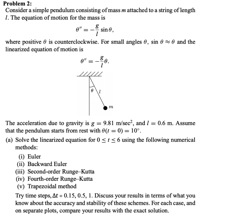
Consider a simple pendulum consisting of mass m attached to a string of length
1. The equation of motion for the mass is
g
0" = — sino,
1 sin
where positive 6 is counterclockwise. For small angles 6, sin 6 ~ 6 and the
linearized equation of motion is
8
0 =-80.
1
[AN]
om
The acceleration due to gravity is g = 9.81 m/sec?, and / = 0.6 m. Assume
that the pendulum starts from rest with 6(t = 0) = 10°.
(a) Solve the linearized equation for 0 < # < 6 using the following numerical
methods:
(i) Euler
(ii) Backward Euler
(iii) Second-order Runge-Kutta
(iv) Fourth-order Runge-Kutta
(v) Trapezoidal method
Try time steps, At = 0.15, 0.5, 1. Discuss your results in terms of what you
know about the accuracy and stability of these schemes. For each case, and
on separate plots, compare your results with the exact solution.
Question:
Problem 2:
Consider a simple pendulum consisting of mass m attached to a string of length
1. The equation of motion for the mass is
g
0" = — sino,
1 sin
where positive 6 is counterclockwise. For small angles 6, sin 6 ~ 6 and the
linearized equation of motion is
8
0 =-80.
1
[AN]
om
The acceleration due to gravity is g = 9.81 m/sec?, and / = 0.6 m. Assume
that the pendulum starts from rest with 6(t = 0) = 10°.
(a) Solve the linearized equation for 0 < # < 6 using the following numerical
methods:
(i) Euler
(ii) Backward Euler
(iii) Second-order Runge-Kutta
(iv) Fourth-order Runge-Kutta
(v) Trapezoidal method
Try time steps, At = 0.15, 0.5, 1. Discuss your results in terms of what you
know about the accuracy and stability of these schemes. For each case, and
on separate plots, compare your results with the exact solution.
This is AI generated Response.
Asked by: Adapaka Jagadeesh
Created at: 2025-07-29 12:13:47
Final Answer:
RenderedRaw Text
Did you like this answer?
Let's break down the steps needed to solve **Problem 2**:
---
### **Step 1: Write the Linearized Equation**
The linearized equation given is:
\[
\theta'' = -\frac{g}{l}\theta
\]
Given:
- \(g = 9.81 \, \text{m/s}^2\)
- \(l = 0.6 \, \text{m}\)
- Initial conditions: \(\theta(0) = 10^\circ = 0.1745 \, \text{rad}\), \(\theta'(0) = 0\)
\[
\frac{g}{l} = \frac{9.81}{0.6} = 16.35
\]
So,
\[
\theta'' + 16.35\theta = 0
\]
---
### **Step 2: Rewrite as First-Order System**
Let \(y_1 = \theta\), \(y_2 = \theta'\):
\[
\begin{cases}
y_1' = y_2 \\
y_2' = -16.35y_1
\end{cases}
\]
with \(y_1(0) = 0.1745\), \(y_2(0) = 0\).
---
### **Step 3: Exact Solution**
The general solution is:
\[
\theta(t) = A\cos(\omega t) + B\sin(\omega t)
\]
where \(\omega = \sqrt{16.35} = 4.042\).
Using initial conditions:
- \(A = 0.1745\)
- \(B = 0\) (since \(\theta'(0) = 0\))
So,
\[
\theta_{\text{exact}}(t) = 0.1745 \cos(4.042 t)
\]
---
### **Step 4: Numerical Schemes**
For each time step (\(\Delta t = 0.15, 0.5, 1\)), solve from \(t=0\) to \(t=6\) seconds.
#### (i) **Euler Method (Forward Euler)**
\[
\begin{cases}
y_1^{n+1} = y_1^n + \Delta t\, y_2^n \\
y_2^{n+1} = y_2^n - \Delta t\, 16.35 y_1^n
\end{cases}
\]
#### (ii) **Backward Euler**
\[
\begin{cases}
y_1^{n+1} = y_1^n + \Delta t\, y_2^{n+1} \\
y_2^{n+1} = y_2^n - \Delta t\, 16.35 y_1^{n+1}
\end{cases}
\]
(Solve as a system for \(y_1^{n+1}\), \(y_2^{n+1}\))
#### (iii) **Second-order Runge-Kutta (RK2, Midpoint)**
\[
k_1 = f(y^n, t^n)\\
k_2 = f(y^n + \frac{\Delta t}{2}k_1, t^n + \frac{\Delta t}{2})\\
y^{n+1} = y^n + \Delta t \cdot k_2
\]
#### (iv) **Fourth-order Runge-Kutta (RK4)**
Standard RK4 steps for the 2D system.
#### (v) **Trapezoidal Method (Crank-Nicolson)**
\[
y^{n+1} = y^n + \frac{\Delta t}{2}(f(y^n, t^n) + f(y^{n+1}, t^{n+1}))
\]
(Again, requires solving a linear system at each step.)
---
### **Step 5: Implementation (Pseudocode)**
For each method, initialize:
- \(y_1^0 = 0.1745\)
- \(y_2^0 = 0\)
- Step through \(t_n = n\Delta t\), update using the method's formula.
---
### **Step 6: Discussion**
#### **Accuracy and Stability**
- **Euler**: Simple but conditionally stable. For oscillatory problems, it can become unstable for large \(\Delta t\).
- **Backward Euler**: More stable (unconditionally for linear systems) but introduces damping (not physical for undamped oscillator).
- **RK2**: Better accuracy, but still conditionally stable.
- **RK4**: High accuracy and stability; preferred for oscillatory problems.
- **Trapezoidal**: Unconditionally stable for linear problems and preserves oscillatory nature better than Backward Euler.
#### **Expected Results**
- For small \(\Delta t\), all methods should closely match the exact solution.
- For larger \(\Delta t\), Forward Euler and RK2 may diverge or dampen; Backward Euler will dampen; Trapezoidal and RK4 will remain accurate and stable.
---
### **Step 7: Plots**
Plot \(\theta(t)\) for each method and \(\Delta t\), and compare against the exact solution.
---
## **Summary Table**
| Method | Stable for Large \(\Delta t\) | Preserves Oscillation | Accuracy | Complexity |
|-----------------|-------------------------------|----------------------|----------|------------|
| Euler | No | No | Low | Low |
| Backward Euler | Yes | No (damps) | Low | Low |
| RK2 | No | No | Medium | Medium |
| RK4 | Yes (for this problem) | Yes | High | Higher |
| Trapezoidal | Yes | Yes | High | Medium |
---
## **What to Submit**
- Code for each method (if required)
- Plots for each method and timestep
- Discussion of accuracy and stability
- Comparison with exact solution
---
If you need example MATLAB/Python code or more detailed explanations for any method, let me know!
VIPSolutions focuses on clear, step‑by‑step explanations so you can learn quickly. Whether you need an AI‑generated walkthrough or a short hint to get unstuck, each solution is organized for fast reading and easy review later.
Search similar questions, compare approaches, and bookmark the best answers for revision. Our goal is simple: quick, reliable study help that feels natural—not noisy.
 VIPSolutions
 Problem 2:
Consider a simple pendulum consisting of mass m attached to a string of length
1. The equation of motion for the mass is
g
0" = — sino,
1 sin
where positive 6 is counterclockwise. For small angles 6, sin 6 ~ 6 and the
linearized equation of motion is
8
0 =-80.
1
[AN]
om
The acceleration due to gravity is g = 9.81 m/sec?, and / = 0.6 m. Assume
that the pendulum starts from rest with 6(t = 0) = 10°.
(a) Solve the linearized equation for 0 < # < 6 using the following numerical
methods:
(i) Euler
(ii) Backward Euler
(iii) Second-order Runge-Kutta
(iv) Fourth-order Runge-Kutta
(v) Trapezoidal method
Try time steps, At = 0.15, 0.5, 1. Discuss your results in terms of what you
know about the accuracy and stability of these schemes. For each case, and
on separate plots, compare your results with the exact solution.