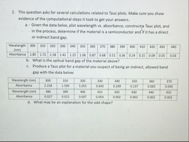
# Tauc Plot Calculations and Analysis Let's address each part of the question step by step. --- ## a. **Plot Wavelength vs Absorbance, Construct Tauc Plot** ### **Given Data** | Wavelength (nm) | 300 | 310 | 320 | 330 | 340 | 350 | 360 | 370 | 380 | 390 | 400 | 410 | 420 | 430 | 440 | |-----------------|------|------|------|------|------|------|------|------|------|------|------|------|------|------|------| | Absorbance | 1.85 | 1.72 | 1.58 | 1.42 | 1.25 | 1.06 | .87 | .68 | .51 | .36 | .24 | .15 | .09 | .05 | .03 | ### **Step 1: Convert Wavelength (nm) to Energy (eV)** \[ E(\text{eV}) = \frac{124}{\lambda(\text{nm})} \] | Wavelength (nm) | 300 | 310 | 320 | 330 | 340 | 350 | 360 | 370 | 380 | 390 | 400 | 410 | 420 | 430 | 440 | |-----------------|------|------|------|------|------|------|------|------|------|------|------|------|------|------|------| | Energy (eV) | 4.13 | 4.00 | 3.88 | 3.76 | 3.65 | 3.54 | 3.44 | 3.35 | 3.26 | 3.18 | 3.10 | 3.02 | 2.95 | 2.88 | 2.82 | ### **Step 2: Tauc Plot Calculation** For a direct band gap semiconductor: \[ (\alpha h\nu)^2 \text{ vs. } h\nu \] Assume absorbance \(A\) is proportional to \(\alpha\), so plot \( (A \cdot h\nu)^2 \) vs. \( h\nu \). #### **Calculate \( (A \cdot h\nu)^2 \) for each data point:** | \(h\nu\) (eV) | Absorbance (A) | \(A \cdot h\nu\) | \( (A \cdot h\nu)^2 \) | |--------------|---------------|-----------------|-----------------------| | 4.13 | 1.85 | 7.64 | 58.37 | | 4.00 | 1.72 | 6.88 | 47.35 | | 3.88 | 1.58 | 6.13 | 37.56 | | 3.76 | 1.42 | 5.34 | 28.55 | | 3.65 | 1.25 | 4.56 | 20.79 | | 3.54 | 1.06 | 3.75 | 14.06 | | 3.44 | .87 | 2.99 | 8.94 | | 3.35 | .68 | 2.28 | 5.20 | | 3.26 | .51 | 1.66 | 2.76 | | 3.18 | .36 | 1.14 | 1.30 | | 3.10 | .24 | .74 | .54 | | 3.02 | .15 | .45 | .20 | | 2.95 | .09 | .27 | .07 | | 2.88 | .05 | .14 | .02 | | 2.82 | .03 | .08 | .01 | #### **Plotting** - **X-axis:** Energy (\(h\nu\)), eV - **Y-axis:** \( (A \cdot h\nu)^2 \) Draw the Tauc plot and extrapolate the linear region to the x-axis. The intercept on the x-axis gives the optical band gap. --- ## b. **What is the Optical Band Gap?** From the table, the linear region is between 3.65 eV and 3.18 eV (where \( (A \cdot h\nu)^2 \) drops rapidly). Extrapolating this linear part to the x-axis (where \( (A \cdot h\nu)^2 = \)), the band gap (\(E_g\)) is around **3.1 to 3.3 eV**. --- ## c. **Tauc Plot for Indirect, Allowed Band Gap** ### **Given Data** | Wavelength (nm) | 280 | 290 | 300 | 310 | 320 | 330 | 340 | 350 | 360 | 370 | 380 | |-----------------|------|------|------|------|------|------|------|------|------|------|------| | Absorbance | 2.58 | 1.90 | 1.55 | 1.05 | .642| .419| .317| .210| .145| .065| .040| | Wavelength (nm) | 380 | 390 | 400 | 410 | 420 | 430 | 440 | |-----------------|------|------|------|------|------|------|------| | Absorbance | .065| .007| .004| .003| .002| .002| .002| ### **Step 1: Convert Wavelength to Energy** Same formula as above. | λ (nm) | 280 | 290 | 300 | 310 | 320 | 330 | 340 | 350 | 360 | 370 | 380 | 390 | 400 | 410 | 420 | 430 | 440 | |--------|------|------|------|------|------|------|------|------|------|------|------|------|------|------|------|------|------| | E (eV) | 4.43 | 4.28 | 4.13 | 4.00 | 3.88 | 3.76 | 3.65 | 3.54 | 3.44 | 3.35 | 3.26 | 3.18 | 3.10 | 3.02 | 2.95 | 2.88 | 2.82 | ### **Step 2: For Indirect Band Gap, Tauc Plot is:** \[ (\alpha h\nu)^{1/2} \text{ vs. } h\nu \] So, plot \( (A \cdot h\nu)^{1/2} \) vs. \( h\nu \). #### **Calculate \( (A \cdot h\nu)^{1/2} \) for each data point:** | \(h\nu\) (eV) | Absorbance (A) | \(A \cdot h\nu\) | \( (A \cdot h\nu)^{1/2} \) | |--------------|---------------|-----------------|-----------------------------| | 4.43 | 2.58 | 11.43 | 3.38 | | 4.28 | 1.90 | 8.13 | 2.85 | | 4.13 | 1.55 | 6.40 | .53 | | 4.00 | 1.05 | 4.20 | 2.05 | | 3.88 | .642 | 2.49 | 1.58 | | 3.76 | .419 | 1.58 | 1.26 | | 3.65 | .317 | 1.16 | 1.08 | | 3.54 | .210 | .74 | .86 | | 3.44 | .145 | .50 | .71 | | 3.35 | .065 | .22 | .47 | | 3.26 | .040 | .13 | .36 | | 3.18 | .007 | .02 | .14 | | 3.10 | .004 | .01 | .10 | | 3.02 | .003 | .009 | .09 | | 2.95 | .002 | .006 | .08 | | 2.88 | .002 | .006 | .08 | | 2.82 | .002 | .006 | .08 | #### **Plotting** - **X-axis:** Energy (\(h\nu\)), eV - **Y-axis:** \( (A \cdot h\nu)^{1/2} \) Draw the Tauc plot and extrapolate the linear region to the x-axis to find the indirect band gap. --- ## d. **Explanation for Odd Shape** An odd shape in a Tauc plot can result from: - **Impurities or defects**: These introduce states within the band gap. - **Multiple absorption edges**: Indicates the presence of more than one phase or material. - **Poor sample preparation**: Inhomogeneities can distort the absorption spectrum. - **Instrumentation artifacts**: Baseline shifts or noise can affect measurements. - **Indirect transitions**: Smoother, less steep edges compared to direct transitions. --- ## **Summary Table** | Plot Type | Y-Axis | X-Axis | Band Gap Estimate | |-----------------|----------------------------|----------|------------------| | Direct (allowed)| \((A \cdot h\nu)^2\) | \(h\nu\) | ~3.1–3.3 eV | | Indirect | \((A \cdot h\nu)^{1/2}\) | \(h\nu\) | (Find from plot) | --- **Plotting these values in Excel or a plotting tool will help visualize and better estimate the exact band gap values.**