 VIPSolutions
Consider the simple linear regression model: Yi=f+hXit+e (a) (3) Assume that X = 0 is within the scope of the model. What is the implication for the regression function if 8p = 07 (b) (4) Under the assumption of Sy = 0, derive the least squares estimate of By. (¢) (6) Find its mean and variance. Ts it unbiased? (d) (2) How do you fit such a model using the Im function? (e) (3) What is the implication for the regression function if 81 = 0? How would the regression function plot on a graph? (f) (4) Under the assumption of 3; = 0, derive the least squares estimate of J3;. (g) (6) Find the Expectation and Variance of the estimate in (f). Is it unbiased ?
Question:
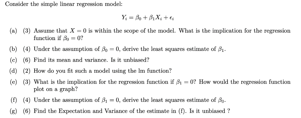 Consider the simple linear regression model:
Yi=f+hXit+e
(a) (3) Assume that X = 0 is within the scope of the model. What is the implication for the regression
function if 8p = 07
(b) (4) Under the assumption of Sy = 0, derive the least squares estimate of By.
(¢) (6) Find its mean and variance. Ts it unbiased?
(d) (2) How do you fit such a model using the Im function?
(e) (3) What is the implication for the regression function if 81 = 0? How would the regression function
plot on a graph?
(f) (4) Under the assumption of 3; = 0, derive the least squares estimate of J3;.
(g) (6) Find the Expectation and Variance of the estimate in (f). Is it unbiased ?
This is AI generated Response.
Asked by: Umesh
Created at: 2025-07-26 22:05:25
Asked by: Umesh
Created at: 2025-07-26 22:05:25
Final Answer:
Rendered
Raw Text
Did you like this answer?
Let's address each part step by step for the simple linear regression model:
\[ Y_i = \beta_0 + \beta_1 X_i + \epsilon_i \]
---
### (a)
**Assume that \( X = 0 \) is within the scope of the model. What is the implication for the regression function if \( \beta_0 = 0 \)?**
**Answer:**
If \( \beta_0 = 0 \), the regression model becomes:
\[ Y_i = \beta_1 X_i + \epsilon_i \]
So, when \( X = 0 \), \( Y = 0 \) (ignoring the error term). This means the regression line passes through the origin. There is no intercept, so for \( X = 0 \), the expected value of \( Y \) is also 0.
---
### (b)
**Under the assumption of \( \beta_0 = 0 \), derive the least squares estimate of \( \beta_1 \).**
**Answer:**
With \( \beta_0 = 0 \), the model is \( Y_i = \beta_1 X_i + \epsilon_i \).
The least squares estimate of \( \beta_1 \) minimizes:
\[
S(\beta_1) = \sum_{i=1}^n (Y_i - \beta_1 X_i)^2
\]
Setting derivative w.r.t. \( \beta_1 \) to zero:
\[
\frac{\partial S}{\partial \beta_1} = -2 \sum_{i=1}^n X_i (Y_i - \beta_1 X_i) = 0
\]
\[
\sum X_i Y_i - \beta_1 \sum X_i^2 = 0 \implies \boxed{\hat{\beta}_1 = \frac{\sum X_i Y_i}{\sum X_i^2}}
\]
---
### (c)
**Find its mean and variance. Is it unbiased?**
**Answer:**
Assume \( Y_i = \beta_1 X_i + \epsilon_i \), \( E[\epsilon_i] = 0 \), \( Var(\epsilon_i) = \sigma^2 \):
- **Expectation:**
\[
E[\hat{\beta}_1] = E\left[\frac{\sum X_i Y_i}{\sum X_i^2}\right] = \frac{\sum X_i E[Y_i]}{\sum X_i^2}
\]
\( E[Y_i] = \beta_1 X_i \), so:
\[
E[\hat{\beta}_1] = \frac{\sum X_i (\beta_1 X_i)}{\sum X_i^2} = \frac{\beta_1 \sum X_i^2}{\sum X_i^2} = \beta_1
\]
**Unbiased**
- **Variance:**
\[
Var(\hat{\beta}_1) = Var\left(\frac{\sum X_i Y_i}{\sum X_i^2}\right) = Var\left(\frac{\sum X_i \epsilon_i}{\sum X_i^2}\right)
\]
Since \( X_i \) are constants,
\[
Var(\hat{\beta}_1) = \frac{\sum X_i^2 Var(\epsilon_i)}{(\sum X_i^2)^2} = \frac{\sigma^2 \sum X_i^2}{(\sum X_i^2)^2} = \frac{\sigma^2}{\sum X_i^2}
\]
---
### (d)
**How do you fit such a model using the lm function?**
**Answer:**
In R, to fit \( Y \sim X - 1 \) (no intercept) using `lm`:
```r
lm(Y ~ X - 1)
```
or
```r
lm(Y ~ 0 + X)
```
---
### (e)
**What is the implication for the regression function if \( \beta_1 = 0 \)? How would the regression function plot on a graph?**
**Answer:**
If \( \beta_1 = 0 \), the model becomes:
\[
Y_i = \beta_0 + \epsilon_i
\]
The regression function is a horizontal line at \( Y = \beta_0 \). On a graph, regardless of \( X \), the regression line is flat at \( \beta_0 \).
---
### (f)
**Under the assumption of \( \beta_1 = 0 \), derive the least squares estimate of \( \beta_0 \).**
**Answer:**
With \( \beta_1 = 0 \), the model is \( Y_i = \beta_0 + \epsilon_i \).
Minimize:
\[
S(\beta_0) = \sum_{i=1}^n (Y_i - \beta_0)^2
\]
Set derivative to zero:
\[
\frac{\partial S}{\partial \beta_0} = -2 \sum (Y_i - \beta_0) = 0
\]
\[
\sum Y_i - n\beta_0 = 0 \implies \boxed{\hat{\beta}_0 = \frac{1}{n} \sum_{i=1}^n Y_i = \bar{Y}}
\]
---
### (g)
**Find the Expectation and Variance of the estimate in (f). Is it unbiased?**
**Answer:**
- **Expectation:**
\[
E[\hat{\beta}_0] = E[\bar{Y}] = \frac{1}{n}\sum E[Y_i] = \frac{1}{n} \sum \beta_0 = \beta_0
\]
So it is **unbiased**.
- **Variance:**
\[
Var(\hat{\beta}_0) = Var(\bar{Y}) = \frac{\sigma^2}{n}
\]
---
Let me know if you need any part explained in more detail!
📢 Instructions:
- Ask anything relatd to above question only.
- For new Question goto :