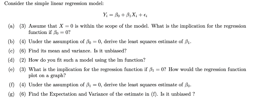
Give step-by-step solution with explanation and final answer:Consider the simple linear regression model:
Yi=f+hXit+e
(a) (3) Assume that X = 0 is within the scope of the model. What is the implication for the regression
function if 8p = 07
(b) (4) Under the assumption of Sy = 0, derive the least squares estimate of By.
(¢) (6) Find its mean and variance. Ts it unbiased?
(d) (2) How do you fit such a model using the Im function?
(e) (3) What is the implication for the regression function if 81 = 0? How would the regression function
plot on a graph?
(f) (4) Under the assumption of 3; = 0, derive the least squares estimate of J3;.
(g) (6) Find the Expectation and Variance of the estimate in (f). Is it unbiased ?
Question:
Give step-by-step solution with explanation and final answer:Consider the simple linear regression model:
Yi=f+hXit+e
(a) (3) Assume that X = 0 is within the scope of the model. What is the implication for the regression
function if 8p = 07
(b) (4) Under the assumption of Sy = 0, derive the least squares estimate of By.
(¢) (6) Find its mean and variance. Ts it unbiased?
(d) (2) How do you fit such a model using the Im function?
(e) (3) What is the implication for the regression function if 81 = 0? How would the regression function
plot on a graph?
(f) (4) Under the assumption of 3; = 0, derive the least squares estimate of J3;.
(g) (6) Find the Expectation and Variance of the estimate in (f). Is it unbiased ?
This is AI generated Response.
Asked by: Umesh
Created at: 2025-07-26 22:29:21
Final Answer:
RenderedRaw Text
Did you like this answer?
Let's go step by step for each part:
### (a) Implication if \( \beta_0 = 0 \) and \( X = 0 \) is within scope
**Given model:**
\[ Y_i = \beta_0 + \beta_1 X_i + \epsilon_i \]
If \( X = 0 \) and \( \beta_0 = 0 \):
- The regression function becomes: \( Y = \beta_1 X \).
- **Implication:** When \( X = 0 \), \( Y = 0 \) (apart from error \( \epsilon \)). Thus, the regression line passes through the origin \((0, 0)\).
---
### (b) Least squares estimate of \( \beta_1 \) when \( \beta_0 = 0 \)
If \( \beta_0 = 0 \), model: \( Y_i = \beta_1 X_i + \epsilon_i \).
**Objective:** Minimize \(\sum_{i=1}^n (Y_i - \beta_1 X_i)^2\)
Take derivative w.r.t. \( \beta_1 \) and set to 0:
\[
\frac{\partial}{\partial \beta_1} \sum_{i=1}^n (Y_i - \beta_1 X_i)^2 = 0
\]
\[
\sum_{i=1}^n -2 X_i (Y_i - \beta_1 X_i) = 0
\]
\[
\sum_{i=1}^n X_i Y_i = \beta_1 \sum_{i=1}^n X_i^2
\]
\[
\boxed{ \hat{\beta}_1 = \frac{ \sum_{i=1}^n X_i Y_i }{ \sum_{i=1}^n X_i^2 } }
\]
---
### (c) Mean, variance, and unbiasedness of \( \hat{\beta}_1 \)
Recall: \( Y_i = \beta_1 X_i + \epsilon_i \), \( E[\epsilon_i] = 0 \), \( Var(\epsilon_i) = \sigma^2 \)
\[
\hat{\beta}_1 = \frac{ \sum_{i=1}^n X_i Y_i }{ \sum_{i=1}^n X_i^2 }
= \frac{ \sum_{i=1}^n X_i (\beta_1 X_i + \epsilon_i) }{ \sum_{i=1}^n X_i^2 }
= \beta_1 \frac{ \sum_{i=1}^n X_i^2 }{ \sum_{i=1}^n X_i^2 } + \frac{ \sum_{i=1}^n X_i \epsilon_i }{ \sum_{i=1}^n X_i^2 }
= \beta_1 + \frac{ \sum_{i=1}^n X_i \epsilon_i }{ \sum_{i=1}^n X_i^2 }
\]
**Expectation:**
\[
E[\hat{\beta}_1] = \beta_1 + \frac{ \sum_{i=1}^n X_i E[\epsilon_i] }{ \sum_{i=1}^n X_i^2 } = \beta_1
\]
So, **it is unbiased**.
**Variance:**
\[
Var(\hat{\beta}_1) = Var\left( \frac{\sum X_i \epsilon_i}{\sum X_i^2} \right) = \frac{Var(\sum X_i \epsilon_i)}{(\sum X_i^2)^2}
\]
Since \( \epsilon_i \) are independent:
\[
Var(\sum X_i \epsilon_i) = \sum X_i^2 Var(\epsilon_i) = \sigma^2 \sum X_i^2
\]
So,
\[
Var(\hat{\beta}_1) = \frac{ \sigma^2 \sum X_i^2 }{ ( \sum X_i^2 )^2 } = \frac{ \sigma^2 }{ \sum X_i^2 }
\]
---
### (d) Fitting such a model using `lm` in R
You fit the model **without an intercept**:
```r
lm(Y ~ X + 0) # or equivalently
lm(Y ~ 0 + X)
```
---
### (e) Implication if \( \beta_1 = 0 \); regression plot
If \( \beta_1 = 0 \):
- Model: \( Y_i = \beta_0 + \epsilon_i \)
- The regression function is flat (horizontal line): \( Y = \beta_0 \).
- **Plot:** A horizontal line at \( Y = \beta_0 \), regardless of \( X \).
---
### (f) Least squares estimate of \( \beta_0 \) when \( \beta_1 = 0 \)
Model: \( Y_i = \beta_0 + \epsilon_i \)
Minimize \( \sum_{i=1}^n (Y_i - \beta_0)^2 \)
Take derivative w.r.t \( \beta_0 \):
\[
\frac{\partial}{\partial \beta_0} \sum_{i=1}^n (Y_i - \beta_0)^2 = -2 \sum_{i=1}^n (Y_i - \beta_0) = 0
\]
\[
\sum_{i=1}^n Y_i = n \beta_0 \implies \boxed{ \hat{\beta}_0 = \frac{1}{n} \sum_{i=1}^n Y_i }
\]
---
### (g) Expectation and variance of \( \hat{\beta}_0 \) in (f). Is it unbiased?
\[
\hat{\beta}_0 = \bar{Y}
\]
\[
E[\bar{Y}] = E\left[\frac{1}{n} \sum Y_i\right] = \frac{1}{n} \sum E[Y_i] = \frac{1}{n} \sum \beta_0 = \beta_0
\]
So, **unbiased**.
\[
Var(\bar{Y}) = \frac{1}{n^2} \sum Var(Y_i) = \frac{1}{n^2} \cdot n \sigma^2 = \frac{\sigma^2}{n}
\]
---
## **Summary Table**
| Part | Solution/Answer |
|------|----------------|
| (a) | Regression passes through origin; at \( X=0, Y=0 \) |
| (b) | \( \hat{\beta}_1 = \frac{\sum X_i Y_i}{\sum X_i^2} \) |
| (c) | Mean: \( \beta_1 \), Variance: \( \frac{\sigma^2}{\sum X_i^2} \), Unbiased: Yes |
| (d) | Use `lm(Y ~ X + 0)` in R |
| (e) | Regression is a horizontal line at \( Y = \beta_0 \) |
| (f) | \( \hat{\beta}_0 = \bar{Y} = \frac{1}{n} \sum Y_i \) |
| (g) | Mean: \( \beta_0 \), Variance: \( \frac{\sigma^2}{n} \), Unbiased: Yes |
Question:
(a) Implication if \(\ce{\beta_0 = 0 }\)\beta_0 = 0 and \(\ce{X = 0 }\)X = 0 is within scope
Given model:
\(\ce{Y_i = \beta_0 + \beta_1 X_i + \epsilon_i If X = 0 and \beta_0 = 0 :}\)Y_i = \beta_0 + \beta_1 X_i + \epsilon_i If X = 0 and \beta_0 = 0 :
The regression function becomes: \(\ce{Y = \beta_1 X }\)Y = \beta_1 X .
Implication: When \(\ce{X = 0 }\)X = 0 , \(\ce{Y = 0 }\)Y = 0 (apart from error \(\ce{\epsilon }\)\epsilon ). Thus, the regression line passes through the origin \(\ce{(0, 0)}\)(0, 0) .
(b) Least squares estimate of \(\ce{\beta_1 }\)\beta_1 when \(\ce{\beta_0 = 0}\)\beta_0 = 0
If \(\ce{\beta_0 = 0 }\)\beta_0 = 0 , model: \(\ce{Y_i = \beta_1 X_i + \epsilon_i }\)Y_i = \beta_1 X_i + \epsilon_i .
Objective:
Minimize \(\ce{\sum_{i=1}^n (Y_i - \beta_1 X_i)^2}\)\sum_{i=1}^n (Y_i - \beta_1 X_i)^2
Take derivative w.r.t. \(\ce{\beta_1 }\)\beta_1 and set to 0:
\(\ce{\frac{\partial}{\partial \beta_1} \sum_{i=1}^n (Y_i - \beta_1 X_i)^2 = 0}\)\frac{\partial}{\partial \beta_1} \sum_{i=1}^n (Y_i - \beta_1 X_i)^2 = 0
\(\ce{\sum_{i=1}^n -2 X_i (Y_i - \beta_1 X_i) = 0}\)\sum_{i=1}^n -2 X_i (Y_i - \beta_1 X_i) = 0
\(\ce{\sum_{i=1}^n X_i Y_i = \beta_1 \sum_{i=1}^n X_i^2}\)\sum_{i=1}^n X_i Y_i = \beta_1 \sum_{i=1}^n X_i^2
\(\ce{ \hat{\beta}_1 = \frac{ \sum_{i=1}^n X_i Y_i }{ \sum_{i=1}^n X_i^2 } }\) \hat{\beta}_1 = \frac{ \sum_{i=1}^n X_i Y_i }{ \sum_{i=1}^n X_i^2 }
explanation in 2 lines
This is AI generated Response.
Asked by: Umesh
Created at: 2025-07-26 22:46:22
Final Answer:
RenderedRaw Text
Did you like this answer?
Let's analyze each part systematically:
**(a) Implication if \( \beta_0 = 0 \) and \( X=0 \) is within scope**
- Model: \( Y_i = \beta_0 + \beta_1 X_i + \epsilon_i \).
- Given \( \beta_0=0 \), the model reduces to \( Y_i = \beta_1 X_i + \epsilon_i \).
- If \( X=0 \) is within the data range (within scope), then at \( X=0 \), the expected value of \( Y \) is \( E[Y] = 0 \), so the regression line passes through the origin.
- **Implication:** The regression function passes through the point \((0,0)\), indicating no intercept.
---
**(b) Least squares estimate of \( \beta_1 \) when \( \beta_0=0 \)**
- Model: \( Y_i = \beta_1 X_i + \epsilon_i \).
- To estimate \( \beta_1 \), minimize the sum of squared residuals:
\[
\min_{\beta_1} \sum_{i=1}^n (Y_i - \beta_1 X_i)^2
\]
- Derivative w.r.t. \( \beta_1 \):
\[
-2 \sum_{i=1}^n X_i (Y_i - \beta_1 X_i) = 0
\]
- Solving for \( \beta_1 \):
\[
\sum X_i Y_i = \beta_1 \sum X_i^2
\]
\[
\boxed{
\hat{\beta}_1 = \frac{\sum_{i=1}^n X_i Y_i}{\sum_{i=1}^n X_i^2}
}
\]
*This is the least squares estimator when intercept is zero.*
---
**(c) Mean, variance, and unbiasedness of \( \hat{\beta}_1 \)**
- Recall: \( Y_i = \beta_1 X_i + \epsilon_i \), with \( E[\epsilon_i]=0 \).
- The estimator:
\[
\hat{\beta}_1 = \frac{\sum X_i Y_i}{\sum X_i^2} = \frac{\sum X_i (\beta_1 X_i + \epsilon_i)}{\sum X_i^2} = \beta_1 + \frac{\sum X_i \epsilon_i}{\sum X_i^2}
\]
- **Expected value:**
\[
E[\hat{\beta}_1] = \beta_1 + \frac{\sum X_i E[\epsilon_i]}{\sum X_i^2} = \beta_1
\]
- **Variance:**
\[
Var(\hat{\beta}_1) = Var\left( \frac{\sum X_i \epsilon_i}{\sum X_i^2} \right) = \frac{1}{(\sum X_i^2)^2} \cdot \sum X_i^2 \sigma^2 = \frac{\sigma^2}{\sum X_i^2}
\]
- **Unbiased?** Yes, because \( E[\hat{\beta}_1] = \beta_1 \).
---
**(d) How to fit such a model using `lm` in R**
- To fit a model **without intercept**:
```r
lm(Y ~ X + 0)
```
or equivalently:
```r
lm(Y ~ 0 + X)
```
This instructs R to estimate the slope **only**, passing through the origin.
---
**(e) Implication if \( \beta_1=0 \)**
- Model reduces to: \( Y_i = \beta_0 + \epsilon_i \).
- The regression is **horizontal** at \( Y = \beta_0 \).
- **Plot:** A flat horizontal line at the mean of Y (if estimated from data).
**Graphically:** The regression line is a straight horizontal line at \( Y = \hat{\beta}_0 \), indicating no relationship between \( X \) and \( Y \).
---
**(f) Least squares estimate of \( \beta_0 \) when \( \beta_1=0 \)**
- Model: \( Y_i = \beta_0 + \epsilon_i \).
- Minimize:
\[
\sum_{i=1}^n (Y_i - \beta_0)^2
\]
- Derivative:
\[
-2 \sum (Y_i - \beta_0) = 0 \Rightarrow \sum Y_i = n \beta_0
\]
- So,
\[
\boxed{
\hat{\beta}_0 = \frac{1}{n} \sum_{i=1}^n Y_i = \bar{Y}
}
\]
---
**(g) Expectation, variance, and unbiasedness of \( \hat{\beta}_0 \)**
- Since \( \hat{\beta}_0 = \bar{Y} \):
\[
E[\hat{\beta}_0] = E[\bar{Y}] = \frac{1}{n} \sum E[Y_i] = \frac{1}{n} \sum (\beta_0 + 0) = \beta_0
\]
- Variance:
\[
Var(\hat{\beta}_0) = Var(\bar{Y}) = \frac{\sigma^2}{n}
\]
- **Unbiased?** Yes, because \( E[\hat{\beta}_0] = \beta_0 \).
---
**Summary:**
| Part | Key Result |
|---------|------------------------------|
| (a) | Regression line passes through origin at \( (0,0) \). |
| (b) | \( \hat{\beta}_1 = \frac{\sum X_i Y_i}{\sum X_i^2} \). |
| (c) | Mean: \( \beta_1 \); Variance: \( \sigma^2 / \sum X_i^2 \); Unbiased: Yes. |
| (d) | Fit with `lm(Y ~ X + 0)` in R. |
| (e) | Regression is a horizontal line at \( Y=\beta_0 \). |
| (f) | \( \hat{\beta}_0 = \bar{Y} \). |
| (g) | Mean: \( \beta_0 \); Variance: \( \sigma^2 / n \); Unbiased: Yes. |
Question:
(a) Implication if \(\ce{\beta_0 = 0 }\)\beta_0 = 0 and \(\ce{X = 0 }\)X = 0 is within scope
Given model:
\(\ce{Y_i = \beta_0 + \beta_1 X_i + \epsilon_i If X = 0 and \beta_0 = 0 :}\)Y_i = \beta_0 + \beta_1 X_i + \epsilon_i If X = 0 and \beta_0 = 0 :
The regression function becomes: \(\ce{Y = \beta_1 X }\)Y = \beta_1 X .
Implication: When \(\ce{X = 0 }\)X = 0 , \(\ce{Y = 0 }\)Y = 0 (apart from error \(\ce{\epsilon }\)\epsilon ). Thus, the regression line passes through the origin \(\ce{(0, 0)}\)(0, 0) .
(b) Least squares estimate of \(\ce{\beta_1 }\)\beta_1 when \(\ce{\beta_0 = 0}\)\beta_0 = 0
If \(\ce{\beta_0 = 0 }\)\beta_0 = 0 , model: \(\ce{Y_i = \beta_1 X_i + \epsilon_i }\)Y_i = \beta_1 X_i + \epsilon_i .
Objective:
Minimize \(\ce{\sum_{i=1}^n (Y_i - \beta_1 X_i)^2}\)\sum_{i=1}^n (Y_i - \beta_1 X_i)^2
Take derivative w.r.t. \(\ce{\beta_1 }\)\beta_1 and set to 0:
\(\ce{\frac{\partial}{\partial \beta_1} \sum_{i=1}^n (Y_i - \beta_1 X_i)^2 = 0}\)\frac{\partial}{\partial \beta_1} \sum_{i=1}^n (Y_i - \beta_1 X_i)^2 = 0
\(\ce{\sum_{i=1}^n -2 X_i (Y_i - \beta_1 X_i) = 0}\)\sum_{i=1}^n -2 X_i (Y_i - \beta_1 X_i) = 0
\(\ce{\sum_{i=1}^n X_i Y_i = \beta_1 \sum_{i=1}^n X_i^2}\)\sum_{i=1}^n X_i Y_i = \beta_1 \sum_{i=1}^n X_i^2
\(\ce{ \hat{\beta}_1 = \frac{ \sum_{i=1}^n X_i Y_i }{ \sum_{i=1}^n X_i^2 } }\) \hat{\beta}_1 = \frac{ \sum_{i=1}^n X_i Y_i }{ \sum_{i=1}^n X_i^2 }
explanation in 2 lines
This is AI generated Response.
Asked by: Umesh
Created at: 2025-07-26 22:49:42
Final Answer:
RenderedRaw Text
Did you like this answer?
Let's analyze each part systematically:
**(a) Implication if \( \beta_0 = 0 \) and \( X=0 \) is within scope**
- Given the model: \( Y_i = \beta_0 + \beta_1 X_i + \epsilon_i \)
- With \( \beta_0=0 \), the model reduces to \( Y_i = \beta_1 X_i + \epsilon_i \).
- Since \( X=0 \) is within the data range, at \( X=0 \), the expected \( Y \) is \( E[Y] = 0 \).
- **Implication:** The regression line passes through the origin \((0,0)\), meaning the intercept is zero, and the predicted \( Y \) is zero when \( X=0 \).
---
**(b) Least squares estimate of \( \beta_1 \) when \( \beta_0=0 \)**
- Model: \( Y_i = \beta_1 X_i + \epsilon_i \)
- To estimate \( \beta_1 \), minimize the sum of squared residuals:
\[
\min_{\beta_1} \sum_{i=1}^n (Y_i - \beta_1 X_i)^2
\]
- Setting derivative to zero:
\[
-2 \sum_{i=1}^n X_i (Y_i - \beta_1 X_i) = 0
\]
\[
\Rightarrow \sum_{i=1}^n X_i Y_i = \beta_1 \sum_{i=1}^n X_i^2
\]
- Solving for \( \beta_1 \):
\[
\boxed{
\hat{\beta}_1 = \frac{\sum_{i=1}^n X_i Y_i}{\sum_{i=1}^n X_i^2}
}
\]
*This is the least squares estimator assuming no intercept.*
---
**(c) Mean, variance, and unbiasedness of \( \hat{\beta}_1 \)**
- Recall: \( Y_i = \beta_1 X_i + \epsilon_i \), with \( E[\epsilon_i]=0 \).
- The estimator:
\[
\hat{\beta}_1 = \frac{\sum X_i Y_i}{\sum X_i^2} = \frac{\sum X_i (\beta_1 X_i + \epsilon_i)}{\sum X_i^2} = \beta_1 + \frac{\sum X_i \epsilon_i}{\sum X_i^2}
\]
- **Expected value:**
\[
E[\hat{\beta}_1] = \beta_1 + \frac{\sum X_i E[\epsilon_i]}{\sum X_i^2} = \beta_1
\]
- **Variance:**
\[
Var(\hat{\beta}_1) = Var\left( \frac{\sum X_i \epsilon_i}{\sum X_i^2} \right) = \frac{1}{(\sum X_i^2)^2} \cdot \sum X_i^2 \sigma^2 = \frac{\sigma^2}{\sum X_i^2}
\]
- **Unbiased?** Yes, because \( E[\hat{\beta}_1] = \beta_1 \).
---
**(d) How to fit such a model using `lm` in R**
- To fit the model **without intercept**:
```r
lm(Y ~ X + 0)
```
or equivalently:
```r
lm(Y ~ 0 + X)
```
This specifies a model passing through the origin.
---
**(e) Implication if \( \beta_1=0 \)**
- The model simplifies to: \( Y_i = \beta_0 + \epsilon_i \).
- The regression line is **horizontal** at \( Y = \hat{\beta}_0 \).
- **Graphically:** The fitted line is a flat horizontal line, indicating **no relationship** between \( X \) and \( Y \).
---
**(f) Least squares estimate of \( \beta_0 \) when \( \beta_1=0 \)**
- Model: \( Y_i = \beta_0 + \epsilon_i \)
- Minimize:
\[
\sum_{i=1}^n (Y_i - \beta_0)^2
\]
- Derivative:
\[
-2 \sum_{i=1}^n (Y_i - \beta_0) = 0 \Rightarrow \sum_{i=1}^n Y_i = n \beta_0
\]
- Therefore,
\[
\boxed{
\hat{\beta}_0 = \frac{1}{n} \sum_{i=1}^n Y_i = \bar{Y}
}
\]
---
**(g) Expectation, variance, and unbiasedness of \( \hat{\beta}_0 \)**
- Since \( \hat{\beta}_0 = \bar{Y} \):
\[
E[\hat{\beta}_0] = E[\bar{Y}] = \frac{1}{n} \sum_{i=1}^n E[Y_i] = \frac{1}{n} \sum_{i=1}^n (\beta_0 + 0) = \beta_0
\]
- Variance:
\[
Var(\hat{\beta}_0) = Var(\bar{Y}) = \frac{\sigma^2}{n}
\]
- **Unbiased?** Yes, because \( E[\hat{\beta}_0] = \beta_0 \).
---
**Summary:**
| Part | Key Result |
|---------|------------------------------|
| (a) | Regression line passes through \((0,0)\). |
| (b) | \( \hat{\beta}_1 = \frac{\sum X_i Y_i}{\sum X_i^2} \) |
| (c) | Mean: \( \beta_1 \); Variance: \( \frac{\sigma^2}{\sum X_i^2} \); Unbiased: Yes. |
| (d) | Fit with `lm(Y ~ X + 0)` in R. |
| (e) | Regression is a flat horizontal line at \( Y=\hat{\beta}_0 \). |
| (f) | \( \hat{\beta}_0 = \bar{Y} \). |
| (g) | Mean: \( \beta_0 \); Variance: \( \frac{\sigma^2}{n} \); Unbiased: Yes. |
**In brief:**
- When \( \beta_0=0 \) and \( X=0 \) is in scope, the line passes through the origin.
- The estimator for \( \beta_1 \) (if intercept is zero) is the ratio of the covariance of \( X \) and \( Y \) over the variance of \( X \).
- Estimators are unbiased with known variance formulas.
VIPSolutions focuses on clear, step‑by‑step explanations so you can learn quickly. Whether you need an AI‑generated walkthrough or a short hint to get unstuck, each solution is organized for fast reading and easy review later.
Search similar questions, compare approaches, and bookmark the best answers for revision. Our goal is simple: quick, reliable study help that feels natural—not noisy.
 VIPSolutions
 Consider the simple linear regression model:
Yi=f+hXit+e
(a) (3) Assume that X = 0 is within the scope of the model. What is the implication for the regression
function if 8p = 07
(b) (4) Under the assumption of Sy = 0, derive the least squares estimate of By.
(¢) (6) Find its mean and variance. Ts it unbiased?
(d) (2) How do you fit such a model using the Im function?
(e) (3) What is the implication for the regression function if 81 = 0? How would the regression function
plot on a graph?
(f) (4) Under the assumption of 3; = 0, derive the least squares estimate of J3;.
(g) (6) Find the Expectation and Variance of the estimate in (f). Is it unbiased ?