 VIPSolutions
(20 points) Consider the following dataset, containing 5 data points: Je _ fo _[-2 _[a _[2 x= alex = | hoxe =| Tx =| xs = of (a) (10 points) What is the first principal component of the data? (b) (10 points) Use PCA to compute lower-dimensional 1-d representations {y, € R : 1
Question:
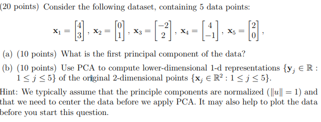 (20 points) Consider the following dataset, containing 5 data points:
Je _ fo _[-2 _[a _[2
x= alex = | hoxe =| Tx =| xs = of
(a) (10 points) What is the first principal component of the data?
(b) (10 points) Use PCA to compute lower-dimensional 1-d representations {y, € R :
1
This is AI generated Response.
Asked by: Umesh
Created at: 2025-08-02 00:06:06
Asked by: Umesh
Created at: 2025-08-02 00:06:06
Final Answer:
Rendered
Raw Text
Did you like this answer?
Let's break down the steps for **Principal Component Analysis (PCA)**:
---
### **Step 1: Write the Data as a Matrix**
Let the data matrix \( X \) be:
\[
X = \begin{bmatrix}
4 & 0 & -2 & 4 & 2 \\
3 & 1 & 2 & -1 & 0
\end{bmatrix}
\]
---
### **Step 2: Center the Data**
Find the mean of each row (dimension):
\[
\text{Mean} =
\begin{bmatrix}
\frac{4 + 0 + (-2) + 4 + 2}{5} \\
\frac{3 + 1 + 2 + (-1) + 0}{5}
\end{bmatrix}
=
\begin{bmatrix}
\frac{8}{5} \\
\frac{5}{5}
\end{bmatrix}
=
\begin{bmatrix}
1.6 \\
1
\end{bmatrix}
\]
Subtract the mean from each column (center the data):
\[
X_{\text{centered}} =
\begin{bmatrix}
4-1.6 & 0-1.6 & -2-1.6 & 4-1.6 & 2-1.6 \\
3-1 & 1-1 & 2-1 & -1-1 & 0-1
\end{bmatrix}
=
\begin{bmatrix}
2.4 & -1.6 & -3.6 & 2.4 & 0.4 \\
2 & 0 & 1 & -2 & -1
\end{bmatrix}
\]
---
### **Step 3: Compute the Covariance Matrix**
\[
\text{Cov}(X) = \frac{1}{n-1} X_{\text{centered}} X_{\text{centered}}^T
\]
where \( n = 5 \).
\[
X_{\text{centered}} X_{\text{centered}}^T =
\begin{bmatrix}
2.4 & -1.6 & -3.6 & 2.4 & 0.4 \\
2 & 0 & 1 & -2 & -1
\end{bmatrix}
\begin{bmatrix}
2.4 & 2 \\
-1.6 & 0 \\
-3.6 & 1 \\
2.4 & -2 \\
0.4 & -1
\end{bmatrix}
\]
Calculate each entry:
- \( a_{11} = 2.4^2 + (-1.6)^2 + (-3.6)^2 + 2.4^2 + 0.4^2 = 5.76 + 2.56 + 12.96 + 5.76 + 0.16 = 27.2 \)
- \( a_{12} = 2.4 \cdot 2 + (-1.6)\cdot 0 + (-3.6)\cdot 1 + 2.4 \cdot (-2) + 0.4 \cdot (-1) = 4.8 + 0 - 3.6 - 4.8 - 0.4 = -4 \)
- \( a_{22} = 2^2 + 0^2 + 1^2 + (-2)^2 + (-1)^2 = 4 + 0 + 1 + 4 + 1 = 10 \)
Symmetric, so \( a_{21} = a_{12} \). Therefore,
\[
X_{\text{centered}} X_{\text{centered}}^T =
\begin{bmatrix}
27.2 & -4 \\
-4 & 10
\end{bmatrix}
\]
Divide by \( n-1 = 4 \):
\[
\text{Cov}(X) = \frac{1}{4}
\begin{bmatrix}
27.2 & -4 \\
-4 & 10
\end{bmatrix}
=
\begin{bmatrix}
6.8 & -1 \\
-1 & 2.5
\end{bmatrix}
\]
---
### **Step 4: Find the First Principal Component (Eigenvector with Largest Eigenvalue)**
Solve \( \det(\text{Cov}(X) - \lambda I) = 0 \):
\[
\begin{vmatrix}
6.8-\lambda & -1 \\
-1 & 2.5-\lambda
\end{vmatrix}
= (6.8-\lambda)(2.5-\lambda) - 1 = 0
\]
\[
(6.8-\lambda)(2.5-\lambda) - 1 = 0
\]
\[
17 - 6.8\lambda - 2.5\lambda + \lambda^2 - 1 = 0
\]
\[
\lambda^2 - 9.3\lambda + 16 = 0
\]
Solve for \( \lambda \):
\[
\lambda = \frac{9.3 \pm \sqrt{9.3^2 - 4 \cdot 1 \cdot 16}}{2}
\]
\[
= \frac{9.3 \pm \sqrt{86.49 - 64}}{2}
= \frac{9.3 \pm \sqrt{22.49}}{2}
= \frac{9.3 \pm 4.75}{2}
\]
So,
- \( \lambda_1 = \frac{9.3 + 4.75}{2} = 7.025 \)
- \( \lambda_2 = \frac{9.3 - 4.75}{2} = 2.275 \)
Take the eigenvector for \( \lambda_1 = 7.025 \):
\[
(\text{Cov}(X) - 7.025 I)\vec{v} = 0
\]
\[
\begin{bmatrix}
-0.225 & -1 \\
-1 & -4.525
\end{bmatrix}
\begin{bmatrix}
v_1 \\
v_2
\end{bmatrix}
= 0
\]
First row: \( -0.225 v_1 - v_2 = 0 \implies v_2 = -0.225 v_1 \)
So eigenvector is proportional to \( \begin{bmatrix} 1 \\ -0.225 \end{bmatrix} \).
Normalize it:
\[
\|\vec{v}\| = \sqrt{1^2 + (-0.225)^2} = \sqrt{1 + 0.050625} = \sqrt{1.050625} \approx 1.025
\]
So normalized:
\[
\mathbf{u}_1 = \frac{1}{1.025} \begin{bmatrix} 1 \\ -0.225 \end{bmatrix} \approx \begin{bmatrix} 0.9756 \\ -0.2196 \end{bmatrix}
\]
---
### **Step 5: Project Data onto First Principal Component**
Let \( \mathbf{u}_1 \) be the first principal component. The 1D representation of each centered data point \( \mathbf{x}_j \) is:
\[
y_j = \mathbf{u}_1^T (\mathbf{x}_j - \text{mean})
\]
For each \( j \):
- \( \mathbf{x}_1 - \text{mean} = \begin{bmatrix} 2.4 \\ 2 \end{bmatrix} \)
- \( \mathbf{x}_2 - \text{mean} = \begin{bmatrix} -1.6 \\ 0 \end{bmatrix} \)
- \( \mathbf{x}_3 - \text{mean} = \begin{bmatrix} -3.6 \\ 1 \end{bmatrix} \)
- \( \mathbf{x}_4 - \text{mean} = \begin{bmatrix} 2.4 \\ -2 \end{bmatrix} \)
- \( \mathbf{x}_5 - \text{mean} = \begin{bmatrix} 0.4 \\ -1 \end{bmatrix} \)
So:
- \( y_1 = 0.9756 \cdot 2.4 + (-0.2196) \cdot 2 = 2.3414 - 0.4392 = 1.9022 \)
- \( y_2 = 0.9756 \cdot (-1.6) + (-0.2196)\cdot 0 = -1.561 \)
- \( y_3 = 0.9756 \cdot (-3.6) + (-0.2196)\cdot 1 = -3.512 - 0.2196 = -3.7316 \)
- \( y_4 = 0.9756 \cdot 2.4 + (-0.2196)\cdot (-2) = 2.3414 + 0.4392 = 2.7806 \)
- \( y_5 = 0.9756 \cdot 0.4 + (-0.2196)\cdot (-1) = 0.39024 + 0.2196 = 0.6098 \)
---
## **Final Answers:**
### (a) **First Principal Component:**
\[
\boxed{
\mathbf{u}_1 \approx \begin{bmatrix} 0.9756 \\ -0.2196 \end{bmatrix}
}
\]
### (b) **Lower-dimensional 1d representations:**
\[
\boxed{
\begin{align*}
y_1 &\approx 1.90 \\
y_2 &\approx -1.56 \\
y_3 &\approx -3.73 \\
y_4 &\approx 2.78 \\
y_5 &\approx 0.61 \\
\end{align*}
}
\]
Let me know if you’d like to see a plot or further steps!
📢 Instructions:
- Ask anything relatd to above question only.
- For new Question goto :