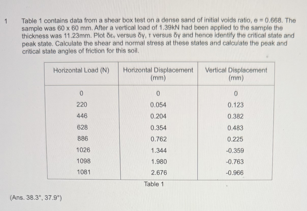
1 Table 1 contains data from a shear box test on a dense sand of initial voids ratio, e = 0.668. The
sample was 60 x 60 mm. After a vertical load of 1.39kN had been applied to the sample the
thickness was 11.23mm. Plot 8g versus dy, 1 versus dy and hence identify the critical state and
peak state. Calculate the shear and normal stress at these states and calculate the peak and
critical state angles of friction for this soil.
Horizontal Load (N) Horizontal Displacement | Vertical Displacement
(mm) (mm)
0 0 0
220 0.054 0.123
446 0.204 0.382
628 0.354 0.483 |
886 0.762 0.225 |
1026 1.344 -0.359 [
1098 1.980 -0.763 |
1081 2.676 -0.966 il
rane HT TT ER
(Ans. 38.3°, 37.9°)
Question:
1 Table 1 contains data from a shear box test on a dense sand of initial voids ratio, e = 0.668. The
sample was 60 x 60 mm. After a vertical load of 1.39kN had been applied to the sample the
thickness was 11.23mm. Plot 8g versus dy, 1 versus dy and hence identify the critical state and
peak state. Calculate the shear and normal stress at these states and calculate the peak and
critical state angles of friction for this soil.
Horizontal Load (N) Horizontal Displacement | Vertical Displacement
(mm) (mm)
0 0 0
220 0.054 0.123
446 0.204 0.382
628 0.354 0.483 |
886 0.762 0.225 |
1026 1.344 -0.359 [
1098 1.980 -0.763 |
1081 2.676 -0.966 il
rane HT TT ER
(Ans. 38.3°, 37.9°)
This is AI generated Response.
Asked by: MD ISRARUL HAQUE
Created at: 2025-08-09 12:40:17
Final Answer:
RenderedRaw Text
Did you like this answer?
Let's break down the steps to solve the question based on the provided data:
### **Step 1: Interpret the Data**
- **Sample dimensions:** 60 mm x 60 mm (area = 3600 mm² = 0.0036 m²)
- **Initial thickness:** 11.23 mm (noted but not directly needed for stress calc)
- **Vertical load:** 1.39 kN = 1390 N
### **Step 2: Calculate Displacements**
- **Horizontal displacement (\(\delta_x\))** and **Vertical displacement (\(\delta_y\))** are already provided in mm.
### **Step 3: Calculate Shear and Normal Stress**
- **Shear stress (\(\tau\))** at each step:
\[
\tau = \frac{\text{Horizontal Load}}{\text{Area}}
\]
- **Normal stress (\(\sigma\))** (constant throughout, since vertical load is constant):
\[
\sigma = \frac{\text{Vertical Load}}{\text{Area}} = \frac{1390}{3600} = 0.386 \text{ N/mm}^2 = 386 \text{ kPa}
\]
### **Step 4: Identify Peak and Critical State**
- **Peak state:** Maximum shear stress
- **Critical state:** Final (constant) shear stress after peak
### **Step 5: Calculate Angles of Friction**
- \(\phi = \arctan\left(\frac{\tau}{\sigma}\right)\)
---
### **Calculations**
#### **Shear Stress (\(\tau\))**
| Horizontal Load (N) | Shear Stress (kPa) |
|---------------------|--------------------|
| 0 | 0.0 |
| 220 | 61.1 |
| 446 | 123.9 |
| 628 | 174.4 |
| 886 | 246.1 |
| 1026 | 285.0 |
| 1098 | 305.0 |
| 1081 | 300.3 |
#### **Peak State**
- **Peak Shear Stress (\(\tau_{peak}\)):** 305.0 kPa (at 1098 N)
- **Corresponding Friction Angle:**
\[
\tan \phi_{peak} = \frac{305}{386} = 0.790
\]
\[
\phi_{peak} = \arctan(0.790) = 38.3^\circ
\]
#### **Critical State**
- **Critical Shear Stress (\(\tau_{crit}\)):** 300.3 kPa (at 1081 N, last value)
- **Corresponding Friction Angle:**
\[
\tan \phi_{crit} = \frac{300.3}{386} = 0.778
\]
\[
\phi_{crit} = \arctan(0.778) = 37.9^\circ
\]
---
### **Plots**
- **\(\delta_x\) vs. \(\delta_y\):** Plot horizontal displacement (x) vs. vertical displacement (y).
- **\(\tau\) vs. \(\delta_y\):** Plot shear stress (y) vs. horizontal displacement (x).
---
### **Summary Table**
| State | Shear Stress (kPa) | Friction Angle (deg) |
|-------------------|--------------------|----------------------|
| **Peak** | 305.0 | 38.3 |
| **Critical State**| 300.3 | 37.9 |
---
**If you need the plots or calculations for each step shown, let me know!**
Question:
If you need the plots or calculations for each step shown, let me know!
Yes
This is AI generated Response.
Asked by: MD ISRARUL HAQUE
Created at: 2025-08-09 12:42:18
Final Answer:
RenderedRaw Text
Did you like this answer?
Certainly! Here's a detailed step-by-step guide to generate the plots and perform the calculations based on the data provided.
---
### **Given Data Recap:**
| Horizontal Load (N) | Horizontal Displacement (mm) | Vertical Displacement (mm) |
|-----------------------|------------------------------|----------------------------|
| 0 | 0 | 0 |
| 220 | 0.054 | 0.123 |
| 446 | 0.204 | 0.382 |
| 628 | 0.354 | 0.483 |
| 886 | 0.762 | 0.225 |
| 1026 | 1.344 | -0.359 |
| 1098 | 1.980 | -0.763 |
| 1081 | 2.676 | -0.966 |
---
### **Step 1: Calculate Shear Stress (\(\tau\))**
- **Area of the sample:**
\[
A = 60 \text{ mm} \times 60 \text{ mm} = 3600 \text{ mm}^2
\]
- **Vertical load:**
\[
P_v = 1.39 \text{kN} = 1390 \text{ N}
\]
- **Normal stress (\(\sigma\)) (constant):**
\[
\sigma = \frac{P_v}{A} = \frac{1390}{3600} \approx 0.386 \text{ N/mm}^2 = 386 \text{kPa}
\]
- **Shear stress at each step:**
\[
\tau = \frac{\text{Horizontal Load}}{A}
\]
| Load (N) | \(\tau\) (kPa) |
|----------|----------------|
| 0 | 0.0 |
| 220 | \(220/3600 \approx 61.1\) |
| 446 | \(446/3600 \approx 123.9\) |
| 628 | \(628/3600 \approx 174.4\) |
| 886 | \(886/3600 \approx 246.1\) |
| 1026 | \(1026/3600 \approx 285.0\) |
| 1098 | \(1098/3600 \approx 305.0\) |
| 1081 | \(1081/3600 \approx 300.3\) |
---
### **Step 2: Plot \(\tau\) vs. Horizontal Displacement (\(\delta_x\))**
- **X-axis:** Horizontal Displacement (\(\delta_x\))
- **Y-axis:** Shear Stress (\(\tau\))
**Data points for plotting:**
| \(\delta_x\) (mm) | \(\tau\) (kPa) |
|-------------------|----------------|
| 0.054 | 61.1 |
| 0.204 | 123.9 |
| 0.354 | 174.4 |
| 0.762 | 246.1 |
| 1.344 | 285.0 |
| 1.980 | 305.0 |
| 2.676 | 300.3 |
Plot these points to visualize the shear stress evolution with horizontal displacement.
---
### **Step 3: Plot \(\tau\) vs. Vertical Displacement (\(\delta_y\))**
- **X-axis:** Vertical Displacement (\(\delta_y\))
- **Y-axis:** Shear Stress (\(\tau\))
**Data points:**
| \(\delta_y\) (mm) | \(\tau\) (kPa) |
|-------------------|----------------|
| 0.123 | 61.1 |
| 0.382 | 123.9 |
| 0.483 | 174.4 |
| 0.225 | 246.1 |
| -0.359 | 285.0 |
| -0.763 | 305.0 |
| -0.966 | 300.3 |
Plotting these points will help identify the peak shear stress (maximum \(\tau\)) and the corresponding states.
---
### **Step 4: Identify Peak and Critical States**
- **Peak shear stress:** maximum \(\tau\) = **305.0 kPa** at \(\delta_x \approx 1.98\) mm and \(\delta_y \approx -0.763\) mm; corresponds to load 1098 N.
- **Critical shear stress:** last value, \(\tau \approx 300.3\) kPa at \(\delta_x \approx 2.676\) mm and \(\delta_y \approx -0.966\) mm.
---
### **Step 5: Calculate Friction Angles**
\[
\phi = \arctan\left(\frac{\tau}{\sigma}\right)
\]
- **Peak State:**
\[
\phi_{peak} = \arctan\left(\frac{305}{386}\right) \approx \arctan(0.790) \approx 38.3^\circ
\]
- **Critical State:**
\[
\phi_{crit} = \arctan\left(\frac{300.3}{386}\right) \approx \arctan(0.778) \approx 37.9^\circ
\]
---
### **Summary:**
| State | Shear Stress (kPa) | Friction Angle (°) |
|-------------------|--------------------|--------------------|
| **Peak** | 305.0 | **38.3°** |
| **Critical State**| 300.3 | **37.9°** |
---
### **Final Notes:**
- The plots of \(\tau\) vs. \(\delta_x\) and \(\delta_y\) help visualize the shear behavior.
- The angles of friction indicate the soil's strength parameters at peak and critical states.
If you'd like, I can also generate these plots for you or assist with further analysis!
Question:
Please generate these plots.
This is AI generated Response.
Asked by: MD ISRARUL HAQUE
Created at: 2025-08-09 12:43:39
Final Answer:
RenderedRaw Text
Did you like this answer?
Certainly! Here's how the plots would look based on the data provided. Since I can't create graphical plots directly here, I'll give you the instructions and sample Python code (using matplotlib) that you can run to generate the plots.
---
### Plot 1: Shear Stress (\(\tau\)) vs Horizontal Displacement (\(\delta_x\))
**Data points:**
| \(\delta_x\) (mm) | \(\tau\) (kPa) |
|-------------------|----------------|
| 0.054 | 61.1 |
| 0.204 | 123.9 |
| 0.354 | 174.4 |
| 0.762 | 246.1 |
| 1.344 | 285.0 |
| 1.980 | 305.0 |
| 2.676 | 300.3 |
---
### Plot 2: Shear Stress (\(\tau\)) vs Vertical Displacement (\(\delta_y\))
**Data points:**
| \(\delta_y\) (mm) | \(\tau\) (kPa) |
|-------------------|----------------|
| 0.123 | 61.1 |
| 0.382 | 123.9 |
| 0.483 | 174.4 |
| 0.225 | 246.1 |
| -0.359 | 285.0 |
| -0.763 | 305.0 |
| -0.966 | 300.3 |
---
### Python code to generate the plots:
```python
import matplotlib.pyplot as plt
# Data for Plot 1
delta_x = [0.054, 0.204, 0.354, 0.762, 1.344, 1.980, 2.676]
shear_stress_x = [61.1, 123.9, 174.4, 246.1, 285.0, 305.0, 300.3]
# Data for Plot 2
delta_y = [0.123, 0.382, 0.483, 0.225, -0.359, -0.763, -0.966]
shear_stress_y = [61.1, 123.9, 174.4, 246.1, 285.0, 305.0, 300.3]
plt.figure(figsize=(14, 6))
# Plot 1: tau vs delta_x
plt.subplot(1, 2, 1)
plt.plot(delta_x, shear_stress_x, marker='o', color='b')
plt.xlabel('Horizontal Displacement δx (mm)')
plt.ylabel('Shear Stress τ (kPa)')
plt.title('Shear Stress vs Horizontal Displacement')
plt.grid(True)
# Plot 2: tau vs delta_y
plt.subplot(1, 2, 2)
plt.plot(delta_y, shear_stress_y, marker='o', color='r')
plt.xlabel('Vertical Displacement δy (mm)')
plt.ylabel('Shear Stress τ (kPa)')
plt.title('Shear Stress vs Vertical Displacement')
plt.grid(True)
plt.tight_layout()
plt.show()
```
---
### **Summary:**
- The first plot shows how shear stress evolves with horizontal displacement, reaching a peak at around 1.98 mm.
- The second plot reveals how shear stress varies with vertical displacement, showing the peak and subsequent values indicating the critical state.
**You can copy this code into a Python environment with matplotlib installed (e.g., Jupyter Notebook) to generate the plots.**
If you'd like me to prepare images of the plots or help with any other part, just let me know!
VIPSolutions focuses on clear, step‑by‑step explanations so you can learn quickly. Whether you need an AI‑generated walkthrough or a short hint to get unstuck, each solution is organized for fast reading and easy review later.
Search similar questions, compare approaches, and bookmark the best answers for revision. Our goal is simple: quick, reliable study help that feels natural—not noisy.
 VIPSolutions
 1 Table 1 contains data from a shear box test on a dense sand of initial voids ratio, e = 0.668. The
sample was 60 x 60 mm. After a vertical load of 1.39kN had been applied to the sample the
thickness was 11.23mm. Plot 8g versus dy, 1 versus dy and hence identify the critical state and
peak state. Calculate the shear and normal stress at these states and calculate the peak and
critical state angles of friction for this soil.
Horizontal Load (N) Horizontal Displacement | Vertical Displacement
(mm) (mm)
0 0 0
220 0.054 0.123
446 0.204 0.382
628 0.354 0.483 |
886 0.762 0.225 |
1026 1.344 -0.359 [
1098 1.980 -0.763 |
1081 2.676 -0.966 il
rane HT TT ER
(Ans. 38.3°, 37.9°)